Difference between revisions of "Taylor Series"
(Created page with '== Single Variable Taylor Series == If we know a function value and its derivatives at some point <var>x</var><sub>0</sub>, we can use a ''Taylor series'' to approximate its val...') |
(Taylor series) |
||
| Line 50: | Line 50: | ||
| + | |||
| + | == Multivariate Taylor Series == | ||
| + | |||
| + | Consider the case where we have several equations that are functions of multiple variables, | ||
| + | :<math> | ||
| + | \begin{array}{c} | ||
| + | f_{1}\left(x_{1},x_{2},\cdots x_{n}\right)\\ | ||
| + | f_{2}\left(x_{1},x_{2},\cdots x_{n}\right)\\ | ||
| + | \vdots \\ | ||
| + | f_{n}\left(x_{1},x_{2},\cdots x_{n}\right)\end{array} | ||
| + | </math> | ||
| + | |||
| + | We can write a multivariate Taylor series expansion for the | ||
| + | <var>i</var><sup>th</sup> function <math>f_i(x_j)</math> as | ||
| + | :<math> | ||
| + | f_{i}(\mathbf{x}) \approx f_{i}(\mathbf{x}_{0}) | ||
| + | + \sum_{j=1}^{n} | ||
| + | + (x_{j}-x_{j0})\frac{\partial f_{i}}{\partial x_{j}} | ||
| + | + \frac{1}{2}(x_{j}-x_{j0})^{2}\frac{\partial^{2}f}{\partial x^{2}} | ||
| + | + \frac{1}{3!}(x_{j}-x_{j0})^{3}\frac{\partial^{3}f}{\partial x^{3}} | ||
| + | + \cdots | ||
| + | </math> | ||
| + | |||
| + | where <math>\mathbf{x}_0</math> is the location where we evaluate the function and <math>n</math> is the number of independent variables. | ||
| + | |||
| + | |||
| + | The term <math>\frac{\partial f_{i}}{\partial x_{j}}</math> is a | ||
| + | matrix called the '''Jacobian''' matrix, <math>[\mathbf{J}]</math> It | ||
| + | is used in solving nonlinear systems of equations using | ||
| + | [[Nonlinear_equations#Newton.27s_Method_for_Systems_of_Equations|Newton's method]]. | ||
| + | |||
| + | |||
| + | === Example === | ||
| + | Consider the equations | ||
| + | :<math> | ||
| + | \begin{cases} | ||
| + | f(x,y) = x^2 + y^2 -1 \\ | ||
| + | g(x,y) = y - x^3 + x - 1 | ||
| + | \end{cases} | ||
| + | </math> | ||
| + | |||
| + | Here <math>n=2</math>. Let's first look at the expansion for <math>f(x,y)</math>. Applying our general equation above we find | ||
| + | :<math> | ||
| + | \begin{align} | ||
| + | f(x,y) \approx f(x_{0},y_{0}) | ||
| + | &+ (x-x_{0})\frac{\partial f}{\partial x} | ||
| + | + \tfrac{1}{2}(x-x_{0})^{2}\frac{\partial^{2}f}{\partial x^{2}} | ||
| + | + \tfrac{1}{6}(x-x_{0})^{3}\frac{\partial^{3}f}{\partial x^{3}} | ||
| + | + \cdots \\ | ||
| + | &+ (y-y_{0})\frac{\partial f}{\partial y} | ||
| + | + \tfrac{1}{2}(y-y_{0})^{2}\frac{\partial^{2}f}{\partial x^{2}} | ||
| + | + \tfrac{1}{6}(y-y_{0})^{3}\frac{\partial^{3}f}{\partial x^{3}} | ||
| + | +\cdots | ||
| + | \end{align} | ||
| + | </math> | ||
| + | The partial derivatives of <math>f(x,y)</math> are: | ||
| + | :{| border=1 cellpadding=10 cellspacing=0 style="text-align:center" | ||
| + | !style="border-bottom:3px solid gray;" | <math>\alpha</math> | ||
| + | !style="border-bottom:3px solid gray;" | <math>\frac{\partial f}{\partial \alpha}</math> | ||
| + | !style="border-bottom:3px solid gray;" | <math>\frac{\partial^2 f}{\partial \alpha^2}</math> | ||
| + | !style="border-bottom:3px solid gray;" | <math>\frac{\partial^3 f}{\partial \alpha^3}</math> | ||
| + | !style="border-bottom:3px solid gray;" | <math>\frac{\partial^4 f}{\partial \alpha^4}</math> | ||
| + | |- | ||
| + | | <math>x</math> || <math>2x</math> || <math>2</math> || 0 || 0 | ||
| + | |- | ||
| + | | <math>y</math> || <math>2y</math> || <math>2</math> || 0 || 0 | ||
| + | |} | ||
| + | substituting this we find | ||
| + | :<math> | ||
| + | f = f(x_0,y_0) | ||
| + | + (x-x_0) 2x + (x-x_0)^2 + (y-y_0) 2y + (y-y_0)^2 | ||
| + | </math> | ||
| + | |||
| + | We can do the same thing for <math>g(x,y)</math> | ||
| + | :<math> | ||
| + | \begin{align} | ||
| + | g(x,y) \approx g(x_{0},y_{0}) | ||
| + | &+ (x-x_{0})\frac{\partial g}{\partial x} | ||
| + | + \tfrac{1}{2}(x-x_{0})^{2}\frac{\partial^{2}g}{\partial x^{2}} | ||
| + | + \tfrac{1}{6}(x-x_{0})^{3}\frac{\partial^{3}g}{\partial x^{3}} | ||
| + | + \cdots \\ | ||
| + | &+ (y-y_{0})\frac{\partial g}{\partial y} | ||
| + | + \tfrac{1}{2}(y-y_{0})^{2}\frac{\partial^{2}g}{\partial x^{2}} | ||
| + | + \tfrac{1}{6}(y-y_{0})^{3}\frac{\partial^{3}g}{\partial x^{3}} | ||
| + | +\cdots | ||
| + | \end{align} | ||
| + | </math> | ||
| + | The partial derivatives of <math>g(x,y)</math> are: | ||
| + | :{| border=1 cellpadding=10 cellspacing=0 style="text-align:center" | ||
| + | !style="border-bottom:3px solid gray;" | <math>\alpha</math> | ||
| + | !style="border-bottom:3px solid gray;" | <math>\frac{\partial g}{\partial \alpha}</math> | ||
| + | !style="border-bottom:3px solid gray;" | <math>\frac{\partial^2 g}{\partial \alpha^2}</math> | ||
| + | !style="border-bottom:3px solid gray;" | <math>\frac{\partial^3 g}{\partial \alpha^3}</math> | ||
| + | !style="border-bottom:3px solid gray;" | <math>\frac{\partial^4 g}{\partial \alpha^4}</math> | ||
| + | |- | ||
| + | | <math>x</math> || <math>-3x^2+1</math> || <math>-6x</math> || -6 || 0 | ||
| + | |- | ||
| + | | <math>y</math> || <math>1</math> || 0 || 0 || 0 | ||
| + | |} | ||
| + | substituting this we find | ||
| + | :<math> | ||
| + | g = g(x_0,y_0) + (x-x_0)(-3x^2+1) + (x-x_0)^2(-3x) + (x-x_0)^3(-x) | ||
| + | + (y-y_0) | ||
| + | </math> | ||
== Multivariate Taylor Series == | == Multivariate Taylor Series == | ||
Revision as of 17:55, 5 August 2009
Contents
Single Variable Taylor Series
If we know a function value and its derivatives at some point x0, we can use a Taylor series to approximate its value at a nearb point x as
If x-x0 is small then we can truncate the series to find
Note that for an nth order polynomial functions, the Taylor series converges in exactly n+1 terms.
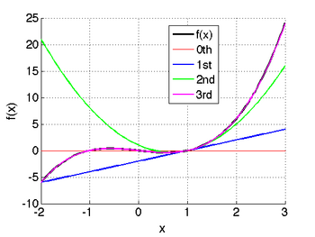
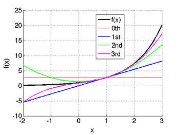
Taylor series approximation of various functions showing the effect of retaining up to 4 terms in the expansion. The expansions are: Note that the third expansion,
 recovers the
function exactly at all points since all higher derivatives (and
therefore all higher terms in the expansion) are zero.
The expansions are: Note that as we retain more terms we become increasingly more accurate. However, this is an infinite series for the exponential function since all of its derivatives are nonzero.
-
Multivariate Taylor Series
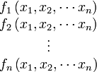
Consider the case where we have several equations that are functions of multiple variables,
We can write a multivariate Taylor series expansion for the
ith function  as
as
where  is the location where we evaluate the function and
  is the number of independent variables.
The term  is a
matrix called the Jacobian matrix,
 ![[\mathbf{J}]](/wiki/images/math/0/a/d/0ad2c2c44fbd9ec9282f5b1769a30c70.png) It
is used in solving nonlinear systems of equations using
Newton's method.
It
is used in solving nonlinear systems of equations using
Newton's method.
Example
Consider the equations
Here  . Let's first look at the expansion for
  . Applying our general equation above we find
The partial derivatives of  are:
are:


0 0 


0 0
substituting this we find
We can do the same thing for 
The partial derivatives of  are:
are:


-6 0 

0 0 0
substituting this we find
Multivariate Taylor Series
Consider the case where we have several equations that are functions of multiple variables,
We can write a multivariate Taylor series expansion for the
ith function  as
as
where  is the location where we evaluate the function and
  is the number of independent variables.
The term  is a
matrix called the Jacobian matrix,
 ![[\mathbf{J}]](/wiki/images/math/0/a/d/0ad2c2c44fbd9ec9282f5b1769a30c70.png) It
is used in solving nonlinear systems of equations using
Newton's method.
It
is used in solving nonlinear systems of equations using
Newton's method.
Example
Consider the equations
Here  . Let's first look at the expansion for
  . Applying our general equation above we find
The partial derivatives of our function are:


0 0 


0 0
substituting this we find


