Difference between revisions of "ODEs"

Revision as of 15:04, 23 February 2009

Solving ODEs in Matlab

To solve an ODE (or a system of ODEs) in Matlab, you need to build a function that evaluates the right-hand-side of the ODEs. For example, let's consider a simple ODE that describes first-order decay

This can easily be separated and solved analytically to find

where is the concentration at .

To solve this in Matlab, we create a function like the following:

function rhs = decay( k, c )
% calculates the rate of decay given the
% rate constant (k) and concentration (c)
rhs = -k*t;

The ODE solvers in Matlab have the following requirements:

• Provide a function that calculates the RHS of the ODE. This function must take two arguments: the independent variable (e.g. time), and the dependent variable(s).
• Provide the time interval over which you desire the solution.
• Provide the value of the dependent variables at the beginning of the time interval (the initial condition).

We can now solve our problem above using the function contained in decay.m to integrate this ODE. The Matlab code to do this is outlined below.

c0 = 10;
k = 0.1;

rhsfun = @(t,c)( decay(k,c) );

[t,c] = ode45( rhsfun, [0,50], c0 );

plot(t,c); xlabel('t'); ylabel('c');

Of course, for this ODE we could solve this without a separate function for the RHS as follows:

c0 = 10;
k = 0.1;
rhs = @(t,c)( -k*c );
[time,conc] = ode45( rhs, [0,50], c0 );
plot(time,conc); xlabel('t'); ylabel('c');

Systems of ODEs in Matlab

Consider a system of ODEs,

To solve a system of ODEs in Matlab, you need to create a function that calculates the RHS of the system as a vector. The function that Matlab's integrator will call to evaluate the RHS must take two arguments:

1. The independent variable. In the system depicted above, this is time,
2. The vector of values of the dependent variable,

In the event that you have a function that requires additional parameters, you can often use an anonymous function to supply these parameters.

Example: Kinetics

Consider the following reactions,

Given , , and initial conditions , , determine the composition of the species as a function of time.

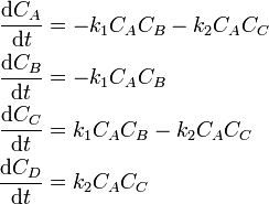
To solve this problem, we need to provide a function that calculates the RHS. We have the following system of ODEs implied by the mechanism:

Reflecting this in Matlab, we have

function rhs = kinetics( c )

% set rate constants
k1 = 1;
k2 = 0.1;

% calculate rates
r1 = k1*c(1)*c(2);
r2 = k2*c(1)*c(3);

% set the rhs.
rhs = zeros(4,1);
rhs(1) = -r1-r2;
rhs(2) = -r1;
rhs(3) = r1-r2;
rhs(4) = r2;

Note that our function has violated the rules for the interface required for Matlab's time integrators mentioned above. We either revise our function, or wrap it with an anonymous function as follows:

% set initial conditions
%      A    B    C  D
c0 = [ 1.0, 0.6, 0, 0 ];

tend = 100;  % ending time for the ODE solution

% build an anonymous function that can be used with Matlab's ODE solver
rhsfun = @(t,c)( kinetics(c) );

% solve the system of ODEs
[t,c] = ode45( rhsfun, [0,tend], c0 );

plot(t,c); xlabel('t'); ylabel('concentration');
legend('A','B','C','D');