Numerical Integration
Contents
Introduction
Numeric integration is used in two general situations:
- we have discrete data and want to integrate it.
- we have an analytic function that we cannot integrate analytically and want to approximate it numerically.
There are many ways to perform numerical integration. We will consider a few here. These are all based on fitting a polynomial function to data and then using what we know about polynomials to obtain the integral.
Midpoint Rule
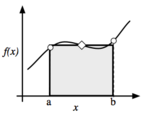
The midpoint rule approximates the integral of a function over some interval [a,b] by a constant. The best choice for the constant value in general will be the function value at the midopoint, (a+b)/2. In other words,
This is shown pictorially in the figure to the right.
Example
Assume that the following flowrate measurements were taken for a river over a 5-day period.
Day 1 2 3 4 5 Flowrate (CFS) 10000 12000 15000 13500 14400
Here the units of flowrate are in cubic feet per second. To get the units consistent, let's convert this into cubic feet per day by multiplying by the number of seconds per day. Then our data becomes
Day 1 2 3 4 5 Flowrate (ft3/day) 8.64x10⁸ 1.049 1.30x10⁹ 1.17x10⁹ 1.24x10⁹
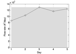
We want to estimate the total volume of water that flowed through the river over this 5-day period. To do this, we could use the flowrate on day 3 (which is the midpoint of the time period) to find
The figure to the right shows this pictorially. However, we can see that the midpoint rule significantly overestimates the total volume (e.g. the integral) since day 3 happened to be the day where the flowrate was highest.
NOTE: the midpoint rule is not always useful for application to discrete data. This is because often the data is not really available at a "midpoint." Therefore, the trapezoid rule is most often used when discrete data needs to be integrated.
Trapezoid Rule
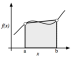
The trapezoid rule uses a linear approximation of the function over the interval [a,b], as shown in the figure to the right. The integral of this is the area of the trapezoid,
Example
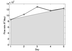
If we apply the trapezoidal rule to the example previously, we use the endpoints of the interval to find
The trapezoid rule is depicted in the figure to the right.
Simpson's 1/3 Rule
|
Example
Summary of Common Quadrature Formulas
| Name | Formula | Comments |
|---|---|---|
| Midpoint Rule | 
|
|
| Trapezoid Rule | ![\int_{a}^{b} f(x) \mathrm{d} x \approx \tfrac{b-a}{2} \left[ f(b)+f(a) \right]](/wiki/images/math/0/f/c/0fc354ac2c1823ba9b99dfa737d052d1.png)
|
|
| Simpson's 1/3 Rule | ![\int_a^b f(x) \mathrm d x \approx \tfrac{\Delta x}{3} \left[ f(a) +4f\left(\tfrac{a+b}{2}\right) + f(b) \right]](/wiki/images/math/e/c/7/ec7275740d9502d428f396e4483e9a06.png)
|
|
Composite Rules: Quadrature
|


![\int_{a}^{b} \approx \frac{b-a}{2} \left[ f(a)+f(b) \right]](/wiki/images/math/9/c/b/9cb10748baeb7557fca416be3494bf30.png)

![\mathrm{Total \; volume} \approx \frac{5-1}{2} \left[ f(1) + f(5) \right] = 2 \cdot \left[ 8.64\times 10^{8} + 1.24\times 10^{9} \right] = 4.22\times 10^{9} \; \mathrm{ft}^3](/wiki/images/math/2/3/d/23d01c502869cf1dbd4cfcd1a0e13e59.png)

![[a,b]](/wiki/images/math/2/c/3/2c3d331bc98b44e71cb2aae9edadca7e.png)
 and
and 