Difference between revisions of "Linear Algebra"
m |
Tilloucifer (talk | contribs) m (LinearAlgebra moved to Linear Algebra: no space!) |
(No difference)
| |
Revision as of 09:57, 2 September 2008
Contents
Basics
Let's first make some definitions:
- Vector
- A one-dimensional collection of numbers. Examples:
-
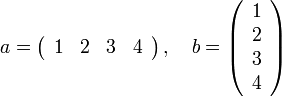
- Matrix
- A two-dimensional collection of numbers. Examples:
-
![A = \left[ \begin{array}{ccc} 1 & 2 & 3 \\ 4 & 5 & 6 \end{array} \right], \quad B = \left[ \begin{array}{cc} 9 & 6 \\ 2 & 3 \end{array}\right]](/wiki/images/math/e/3/1/e31fbd232103b5566994240f6b1d71d5.png)
- Array
- An n-dimensional collection of numbers. A vector is a 1-dimensional array while a matrix is a 2-dimensional array.
- Transpose
- An operation that involves interchanging the rows and columns of an array. It is indicated by a
 superscript. For example:
 -
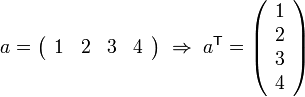
-
![A = \left[ \begin{array}{ccc} 1 & 2 & 3 \\ 4 & 5 & 6 \end{array} \right] \; \Rightarrow \;
A^\mathsf{T} = \left[ \begin{array}{cc} 1 & 4 \\ 2 & 5 \\ 3 & 6 \end{array} \right]](/wiki/images/math/b/d/e/bde86d6b22070666317b8fb53c9a16ae.png)
- Vector Magnitude,

- A measure of the length of a vector,
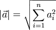
- Example:

- Example:

Matrix & Vector Algebra
There are many common operations involving matrices and vectors including:
These are each discussed in the following sub-sections.
Vector Dot Product
The dot product of two vectors produces a scalar. Physically, the dot product of a and b represents the projection of a onto b.
Given two vectors a and b, their dot product is formed as
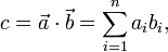
where  and
and  are the components in vectors a and b respectively. This is most useful when we know the components of the vectors a and b.
Occasionally we know the magnitude of the two vectors and the angle between them. In this case, we can calculate the dot product as
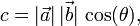
where θ is the angle between the vectors a and b.
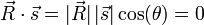
Note that if a and b are both column vectors, then  .
.
For more information on the dot product, see wikipedia's article.
Dot Product in MATLAB
There are several ways to calculate the dot product of two vectors in MATLAB:
  c = dot(a,b);
  c = a' * b;    % if a and b are both column vectors.
Thought examples
Consider the cartoon shown to the right.
- At noon, when the sun is directly overhead, a rocket is launched directly toward the sun at 1000 mph. How fast is its shadow moving?
- Define the rocket's velocity as
 .
. - Define the unit normal on the ground (i.e. the direction of the rocket's shadow on the ground) as
 , where
  .
. - Intuition tells us that if the it is moving directly toward the sun, then its shadow does not appear to move at all. : The dot product
 since cos(90°)=0.
- Consider the same rocket going parallel to the earth's surface. How fast is its shadow moving?
- If the rocket is going parallel to the earth's surface, our intuition tells us that is shadow is moving at the same speed. This is confirmed by the mathematics, since the angle between the rocket's path and the ground is 0. Therefore, since cos(0°)=1.
- What if the rocket were going at a 45° angle?
- Our intuition tells us that the shadow will appear to move, but it will not be moving as fast as the rocket is moving. Mathematically, we have
 .
.
Vector Cross Product
The cross product of two vectors produces a vector perpendicular to the original two. The common right-hand rule is used to determine the direction of the resulting vector.

Assume that we have vectors a and b defined as
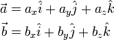
where  ,
,  , and
, and  represent the unit-normal vectors in the x, y, and z directions, respectively.
The cross product of a and b is then defined as
represent the unit-normal vectors in the x, y, and z directions, respectively.
The cross product of a and b is then defined as

If we know the magnitude of a and b and the angle between them (θ), then the cross-product is given as
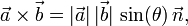
where n is the unit-normal vector perpendicular to the plane defined by the vectors a and b.
For more information, see wikipedia's article on the cross product.
Vector Cross Product in MATLAB
c = cross(a,b); % c is a vector!
Matrix-Vector Product
The matrix-vector product is frequently encountered in solving linear systems of equations, although there are many other uses for it.
Consider a matrix A with m rows and n columns and vector b with n rows:
![A=\left[\begin{array}{cccc}
a_{11} & a_{12} & \cdots & a_{1n}\\
a_{21} & a_{22} & \cdots & a_{2n}\\
\vdots & \vdots & \ddots & \vdots\\
a_{m1} & a_{m2} & \cdots & a_{mn}\end{array}\right],
\quad
b=
\left(\begin{array}{c}
b_{1}\\ b_{2}\\ \vdots\\ b_{n}
\end{array}\right)](/wiki/images/math/5/a/c/5ac41a50c2f681b1cb7b3641e692b7e0.png)
We may multiply A and b if the number of columns in A is equal to the number of rows in b. The product, c is a vector with m rows. The ith entry in c is given as
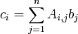
For example, let's consider the following case:
![A = \left[\begin{array}{ccc}
1 & 3 & 2 \\
2 & 5 & 4
\end{array}\right],
\quad
b = \left(\begin{array}{c}
10 \\ 4 \\ 6
\end{array} \right)](/wiki/images/math/0/9/a/09a75f9e23e7be0954f36ecd4d99a351.png)
Here we have m=2 and n=3. We define the product, c=Ab, as follows:
- Be sure that A and b are compatible for multiplication.
- Since A has three columns and b has three rows, they are compatible.
- Determine how many entries are in c.
- The c vector will have as many rows as A has.
- Since A has two rows, c will have two rows.
- Determine the elements in c
- Applying the above formula for i=1 we find
- Applying the above formula for i=2 we find
- Applying the above formula for i=1 we find
Therefore, we have
Matrix-Vector product in MATLAB
c = A*b; % A is a matrix, b and c are vectors.
Matrix-Matrix Product
The matrix-matrix product is a generalization of the matrix-vector product. Consider the general case where we want to multiply two matrices, C = A B, where A and B are matrices. The following rules apply:
- The number of columns in A must be equal to the number of rows in B.
- The number of columns in C is equal to the number of columns in B.
- The number of rows in C is equal to the number of rows in A.
We can state this differently. Suppose that A has m rows and p columns, and that B has p rows and n columns. This satisfies rule 1 above. Then, according to rules 2 and 3, C has m rows and n columns.
The general formula for matrix multiplication is
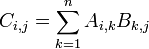
Let's show how this works for a simple example:
![A = \left[ \begin{array}{cc}
1 & 2 \\ 3 & 5
\end{array} \right],
\quad
B = \left[ \begin{array}{ccc}
2 & 4 & 10 \\ 6 & 3 & 1
\end{array} \right].](/wiki/images/math/a/3/3/a33807c3ad2ce2feda2960f4caecbe84.png)
We can form C=A B since rule 1 is satisfied. From the size of A and B we define m=2 and n=3 and from rules 2 and 3, we conclude that the resulting matrix, C has 2 rows and 3 columns.
We are now ready to build each element of C.
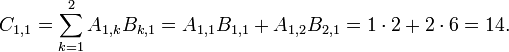
- i=1 and j=1
-
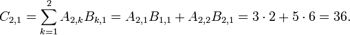
- i=2 and j=1
-
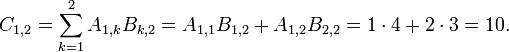
- i=1 and j=2
-
- i=2 and j=2
-
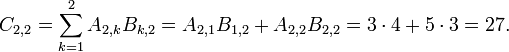
- i=1 and j=3
-

- i=2 and j=3
-
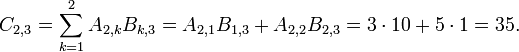
Now, putting all of these together, we have
![C=\left[\begin{array}{ccc}
14 & 10 & 12 \\
36 & 27 & 35
\end{array}\right].](/wiki/images/math/8/1/9/8197065e460efa184aa2ac872f7e37da.png)
Matrix-Matrix product in MATLAB
C = A*B; % A, B, and C are all matrices.
The MATLAB code to implement the above example is
   A = [ 1 2; 3 5; ];
   B = [ 2 4 10; 6 3 1; ];
   C = A*B;
Linear Systems of Equations
Any set of linear systems may be written in the form =(b)](/wiki/images/math/b/3/a/b3ae30ff4dcdb54b97d86d814ca503d6.png) , where
, where ![[A]](/wiki/images/math/7/e/2/7e2bf8880d46cb84f91d8740b2659a88.png) is a matrix and
is a matrix and  and
and  are vectors. In general, for a system of equations with n unknowns x1 ... xn, can be written as
where  and are numbers and
  is the set of unknown variables. These equations can now be written in matrix format:
![\left[ \begin{array}{ccccc}
a_{1,1} & a_{1,2} & a_{1,3} & \cdots & a_{1,n} \\
a_{2,1} & a_{2,2} & a_{2,3} & \cdots & a_{2,n} \\
\vdots & \vdots & \ddots & \vdots & \vdots \\
a_{n,1} & a_{n,2} & a_{n,3} & \cdots & a_{n,n}
\end{array} \right]
\left( \begin{array}{c} x_1 \\ x_2 \\ \vdots \\ x_n \end{array} \right)
=
\left( \begin{array}{c} b_1 \\ b_2 \\ \vdots \\ b_n \end{array} \right).](/wiki/images/math/6/4/2/642696f07ee1eeb0986341fbd1b6e34a.png)
Example
Consider the following equations:
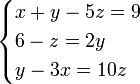
To put these in matrix format, we first choose the solution vector. Let's choose to order this as x, y, z. Now we rewrite the original system so that we have a coefficient multiplying each of these variables, and then we put the "constant" on the right-hand-side:
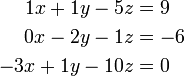
We may then identify the A matrix and b vectors and write
![\left[\begin{array}{ccc}
1 & 1 & -5 \\
0 & -2 & -1 \\
-3 & 1 & -10 \\
\end{array} \right]
\left( \begin{array}{c}
x \\ y \\ z
\end{array}\right)
=
\left( \begin{array}{c}
9 \\ -6 \\ 0
\end{array}\right)](/wiki/images/math/b/f/8/bf8e5ba530c6d522f80f30e36806149e.png)
Note that if we multiply the above matrix and vector, we recover the original set of equations (try it to be sure that you can do it).
Note that if we chose a different variable ordering, then it simply rearranges the columns in the matrix. For example, if we order the variables z, x, y then we have
![\begin{align}
-5z + 1x + 1y &= 9 \\
-1z + 0x - 2y &= -6 \\
-10z - 3x + 1y &= 0
\end{align}
\quad \Rightarrow \quad
\left[\begin{array}{ccc}
-5 & 1 & 1 \\
-1 & 0 & -2 \\
-10 & -3 & 1 \\
\end{array} \right]
\left( \begin{array}{c}
z \\ x \\ y
\end{array}\right)
=
\left( \begin{array}{c}
9 \\ -6 \\ 0
\end{array}\right)](/wiki/images/math/2/3/7/2371c4f3d9f6d52b195e09e4fba2cf55.png)
Solving Linear Systems of Equations
|
Direct Solvers
Gaussian Elimination
The Thomas Algorithm (Tridiagonal Systems)
Iterative Solvers
Jacobi Method
Gauss-Seidel Method
Other Methods
- Conjugate-Gradient
- GMRES