Matlab Arrays

Array Basics

An array is an n-dimensional collection of numbers. Matrices are 2-dimensional arrays, and vectors are 1-dimensional arrays.

Vectors can be either a row or column vector:

$\quad a= \begin{bmatrix} a_1 \\ a_2 \\ a_3 \\ \vdots \\ a_n \end{bmatrix} \quad b = \begin{bmatrix} b_1 & b_2 & \cdots & b_n \end{bmatrix} \quad c = \begin{bmatrix} 1 \\ 4 \\ 3.2 \\ \pi \end{bmatrix}$

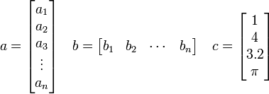
We refer to the elements of an array by their position in the array. For example, the third element in $c$ is 3.2, and the second element in $a$ is $a_2$.

Matrices are two-dimensional arrays, whose elements are referred to by the row and column that they belong to. For example,

$\quad A = \begin{bmatrix} a_{11} & a_{12} \\ a_{21} & a_{22} \\ a_{31} & a_{32} \end{bmatrix}$

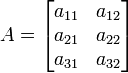
is a matrix with three rows and two columns. We refer to this as a $\scriptstyle 3 \times 2$ matrix. The first index refers to the row and the second index refers to the column.

Transposing Arrays

Occasionally we want to transpose an array. This is done by exchanging rows and columns. For example,

$A = \begin{bmatrix} 2 & 4 \\ 6 & 8 \\ 10 & 12 \end{bmatrix} \quad \Rightarrow \quad A^\mathsf{T} = \begin{bmatrix} 2 & 6 & 10 \\ 4 & 8 & 12 \end{bmatrix}$

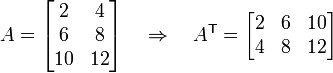
Here the $^\mathsf{T}$ superscript indicates transpose. Note that if we transpose an array twice, we recover the original array. In other words, $\left(A^\mathsf{T}\right)^\mathsf{T} = A$.

Creating Arrays in Matlab

In this section we will discuss several ways of creating arrays (matrices and vectors) in MATLAB.

Manual Creation

Often we need to create small arrays with only a few numbers. In this case, it is easiest to create the vector in one Matlab statement. For example, to create the column vector

$a = \begin{bmatrix} 2 \\ 4 \\ 6 \\ 8 \end{bmatrix}$

we could use any of the following Matlab commands:

 a = [ 2; 4; 6; 8; ];  % create a column vector
 a = [ 2 4 6 8 ]';     % create a row vector and then
                       % transpose it to produce a column vector.
 a = [ 2
       4
       6
       8 ];  % creates a column vector.

Note that the semicolon (;) identifies the end of a row in the matrix. Commas may be used to separate columns in the matrix, but they are not necessary.

A row vector such as b = [1 3 5 7 ] may be created as

  b = [ 1 3 5 7 ];
  b = [ 1, 3, 5, 7 ];
  b = [ 1; 3; 5; 7 ]';  % transpose a column vector.

Matrices may be created directly in much the same way as vectors are. As an example, let's build the matrix

$A = \begin{bmatrix} 2 & 4 \\ 6 & 8 \\ 10 & 12 \end{bmatrix}.$

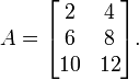
This may be done in several ways.

  A = [ 2 4; 6 8; 10 12 ];
  A = [ 2 4
        6 8
        10 12 ];

Note that a semicolon (;) separates each row of the matrix while spaces separate each column.

We may also create a matrix from vectors. For example, we may construct A from its rows as follows:

  arow1 = [ 2 4 ];
  arow2 = [ 6 8 ];
  arow3 = [ 10 12 ];
  A = [ arow1; arow2; arow3 ];

Similarly, we can build a matrix from its columns:

  acol1 = [2 6 10]';
  acol2 = [4; 8; 12];
  A = [ acol1 acol2 ];

Using the ":" operator to create arrays

Sometimes we have vectors that have specific patterns. For example, a=[1 2 3 4 5]. The : operator (see here for MATLAB's explanation of this) can help us create such arrays:

  array = lower : increment : upper;

This creates an array starting at lower and ending at upper with spacing of increment. You may eliminate the increment argument, in which case it defaults to 1.

Examples:

  a = 1:5;        % creates a=[ 1 2 3 4 5 ]
  b = 1:1:5;      % creates b=[ 1 2 3 4 5 ]
  c = 1:2:7;      % creates c=[ 1 3 5 7 ]
  d = 1:2:8;      % creates d=[ 1 3 5 7 ]
  e = 1.1:5       % creates e=[ 1.1 2.3 3.1 4.1 ]
  f = 0.1:0.1:0.5 % creates f=[ 0.1 0.2 0.3 0.4 0.5 ]
  g = 5:-1:1;     % creates g=[ 5 4 3 2 1 ];
  h = (1:3)';     % creates a column vector with elements 1, 2, 3.

Linspace and Logspace

Occasionally we want to create numbers that are equally spaced between two limits. We can use the linspace command to do this.

linspace( lo, hi, n );

Creates a row vector with n points equally spaced between lo and hi.

The last argument, n is not required. If omitted, 100 points will be used.

Examples:

  a = linspace(1,5,5);    % creates a=[ 1 2 3 4 5 ]
  b = linspace(1,5,4);    % creates b=[ 1.0 2.333 3.667 5.0 ]
  c = linspace(5,1,5);    % creates c=[ 5 4 3 2 1 ]
  d = linspace(1,5,5)';   % creates a column vector
  e = linspace(1,5);      % uses 100 points between 1 and 5.
  lo=0; hi=10;
  f = linspace(lo,hi);    % uses 100 points between lo (0) and hi (10)

Sometimes we want points logarithmically spaced. For example, we may want to create a vector a=[ 0.1 1 10 100]. This can be accomplished using the logspace command:

logspace( lo, hi, n );

Creates a vector with n points spaced logarithmically between $10^\mathrm{lo}$ and $10^\mathrm{hi}$

The last argument, n is not required. If omitted, 50 points will be used.

Examples:

  a = logspace(-1,3,5);    % creates a=[ 0.1 1 10 100 1000 ]
  b = logspace(3,-1,5);    % creates b=[ 1000 100 10 1 0.1 ]
  c = logspace(-1,3,5)';   % creates a column vector
  d = logspace(-3,3);      % 50 points between 10^-3 and 10^3.

Shortcuts for Special Matrices

ones(nrow,ncol) [1]

creates an array of all ones with nrow rows and ncol columns.

zeros(nrow,ncol) [2]

creates an array of all zeros with nrow rows and ncol columns.

eye(nrow,ncol) [3]

creates an array with ones on its diagonal and zeros elsewhere.

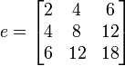
Example: eye(3,2) produces $\begin{bmatrix} 1 & 0 \\ 0 & 1 \\ 0 & 0 \end{bmatrix}$ while eye(3,3) gives $\begin{bmatrix} 1 & 0 & 0 \\ 0 & 1 & 0\\ 0 & 0 & 1 \end{bmatrix}$

rand(nrow,ncol) [4]

creates an array with nrow rows and ncol columns full of random numbers.

Sparse Matrices

This section is a stub and needs to be expanded. If you can provide information or finish this section you're welcome to do so and then remove this message afterwards.

Array Arithmetic

One of the most powerful features of MATLAB is the ability to perform operations on entire arrays at once.

Addition and Subtraction

Given two arrays of the same size, one may add or subtract these as follows:

  C = A + B;

Example 1:

  A = rand(3);
  B = ones(3);
  C = A+B;
  D = B + eye(3);

Example 2:

  a = [1 2 3];
  b = [4 5 6];
  c = a+b;
  d = a' + b';

Example 3:

  A = [1 2 3; 4 5 6];
  a = [-1 -2 -3];
  b = a + A(1,:);

Multiplication

Multiplication of two arrays, C=A*B requires that the number of columns in A is equal to the number of rows in B. The array C has the same number of rows as A and same number of columns as B.

Example 1 - Here A and B are the same size:

  A = rand(3); B = rand(3);
  C = A*B;

Example 2 - Here b is a vector and the product is also a vector.

  A = rand(3);  b = rand(3,1);
  c = A*B;

Example 3 - Here A and B are both matrices, but of different size.

  A = rand(3,5);
  B = rand(5,2);
  C = A*B;

C is a 3x2 array (3 rows, 2 columns)

Elemental Operations

The following table summarizes the elemental operators available in MATLAB. Each of these operators is discussed in more detail below.

Summary of Elemental Operations

Operator	Description
.*	Elemental Multiplication
./	Elemental Division
.^	Elemental Exponentiation

Elemental Multiplication

Arrays of the same size may be multiplied or divided element-by-element using the .* operator so that C = A .* B produces an array whose elements are given by 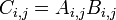$C_{i,j} = A_{i,j} B_{i,j}$.

Example 1:

  A = [1 2; 3 4];
  B = 2*ones(2);
  C = A .* B

This results in $C = \begin{bmatrix} 2 & 4 \\ 6 & 8 \end{bmatrix}$

Example 2:

  a = [1 2 3];
  b = [2; 4; 6];
  c = a .* b';

This results in 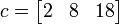$c = \begin{bmatrix} 2 & 8 & 18 \end{bmatrix}$. Note that elemental multiplication is very different from array multiplication. For example,

  d = a*b;
  e = b*a;

would produce d = 24, and $e = \begin{bmatrix} 2 & 4 & 6 \\ 4 & 8 & 12 \\ 6 & 12 & 18 \end{bmatrix}$.

If you need to brush up on this, see the tutorial on matrix multiplication.

Elemental Division

The . / operator performs elemental division on two arrays of the same size.

Example 1:

  a = [ 2 4 6 ];
  b = [ 1 2 3 ];
  c = a./b;
  d = b./a;

results in c=[2 2 2] and d=[0.5 0.5 0.5].

Example 2:

  A = [1 2 3; 4 5 6];
  B = rand(2,3);
  C = A./B;
  D = B./A;

Elemental Exponentiation

A .^ b results in each element in A being raised to the power b. Here b must be a scalar, not a matrix or a vector.

Example 1:

  x = linspace(-pi,pi);
  y = sin(x);
  z = cos(x);
  w = y.^2 + z.^2;

Here all elements of w should be equal to 1.

NOTE: Elemental exponentiation is very different from array exponentiation. For example:

  A = [1 2; 3 4];
  B = A.^3;
  C = A^3;

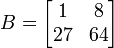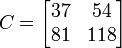results in $B = \begin{bmatrix} 1 & 8 \\ 27 & 64 \end{bmatrix}$ and $C = \begin{bmatrix} 37 & 54 \\ 81 & 118 \end{bmatrix}$. Here we have C=A*A*A, where these are matrix-matrix multiplications.

Accessing Arrays

Often we need to access certain elements or groups of elements from an array. There are a few ways to do this.

Indexing arrays

Recall that an array is simply a collection of numbers. Arrays may be 1-dimensional (vectors), 2-dimensional (matrices) or even higher dimensional. Each number in an array has a unique location identified by an index. Array indexing is best illustrated by example.

  a = 2:2:10;  % creates a row vector: [2 4 6 8 10]
  a1 = a(1);   % assigns the first element of a to "a1"

We can likewise index into a matrix as:

  B = [ 5 2 9; 1 7 3; 2 6 0];
  var = B(2,3);      % var = 3  (row 2, column 3)

In general for a two-dimensional array, B(i,j) refers to the i^th row and j^th column of B. This is extensible to arrays of higher dimensions as well.

If we return to our previous example with the B matrix, we find something interesting:

  B = [ 5 2 9; 1 7 3; 2 6 0];
  b = B(5);

What should the value of b be? One might expect this to result in an error, since B is not a vector. However, this returns b=7. What is happening? Matlab actually treats a matrix as a long vector, B = [ 5 2 9 1 7 3 2 6 0 ], with each row stacked next to the previous row. Therefore, B(5) says "go to the fifth entry" counted along rows.

Slicing arrays using the ":" operator

Sometimes we need to grab a group of elements from an array. We can do this using the : operator For example:

  A = [ 1 2 3; 4 5 6; 7 8 9 ];
  col1 = A(:,1);  % all rows, first column
  row2 = A(2,:);  % second row, all columns

Here : acts to select all elements in the row or column of A. We can grab a subset of rows or columns by the following:

  A = [ 1 2 3; 4 5 6; 7 8 9 ];
  a = A( 1:2, 2:3 );

This takes rows 1 and 2 and columns 2 and 3 in A and creates a new array a. Now a looks like $a=\begin{bmatrix}2 & 3 \\ 5 & 6 \end{bmatrix}$.

The : operator is a very powerful tool to extract portions of an array.

Information about Arrays

size

returns the number of rows and columns in an array. For example,

A = [1 2 3; 4 5 6];

[nrow,ncol] = size(A);

The result of this is that nrow=2 and ncol=3.

length

returns the number of elements in a vector. Example:

a = [1 2 3 4 3 2 1];

na = length(a);

Results in na=7.

max

For a vector, max(v) returns the largest element in v. For matrices, max(V) returns a row vector whose elements contain the maximum value in each column of V.

min

Analogous to max.

Other Useful Tools

Use MATLAB's help command to learn more about how to use these commands.

Matlab command	Summary	Example(s)
sum	For a vector, sum(v) returns the sum of the elements of v. For matrices, sum(V) returns a row vector whose elements contain the sum of the columns of V.	a=sum([1 2 3]); % a=6 b=sum([1 2; 3 4]); % b = [4 6]
sort	Sort an array in ascending or descending order.	sort([2 5 1]) % gives '''1 2 5'''
any	any(A) Evaluates to "true" if any of the elements in the array are true (nonzero).	a=[1 2 3]; b=[1 3 4]; r1 = any(a>b); % r1 is FALSE (equal to 0) r2 = any(a==b); % r2 is TRUE (equal to 1) since a(1) is equal to b(1).
all	Evaluates to "true" if all of the elements in the array are true (nonzero).	A = [1 2; 3 4]; B = [-1 1; 2 3]; r1 = all(A>B); % r1 is TRUE (equal to 1) since the elements in A are % all greater than their corresponding elements in B. r2 = all(2*B>A); % r2 is FALSE
find	find(A) returns the indices where A is nonzero.	A = [1 5 0; 0 2 0]; i = find(A(:,1)); % i=1 i = find(A(:,2)); % i=[1 2]' i = find(A); % i=[1 3 4]' [i,j] = find(A); % i=[ 1 1 2 ]' j=[ 1 2 2 ]' i = find(A>4); % i=3 [i,j] = find(A<2); % i=[1 2 1 2]' j=[1 1 3 3]'
isequal	isequal(A,B) returns true if all elements of A and B are equal, false otherwise.	A = [1 2; 3 4]; B = [2 4; 6 8]; c = isequal(A,B); % c is FALSE d = isequal(2*A,B); % d is TRUE Here is something a bit more complex, using the fact that $\sin^2(\alpha)+\cos^2(\alpha) = 1$ x = rand(5); y1 = sin(x).*sin(x); z1 = cos(x).*cos(x); q = ones(5); c = isequal(q,y1+z1); % c is TRUE