Difference between revisions of "Nonlinear equations"
m (→Closed Domain Methods === {{Stub|section}} ==== Bisection =) |
|||
| Line 1: | Line 1: | ||
== Introduction == | == Introduction == | ||
| − | |||
| + | Nonlinear equations arise ubiquitously in science and engineering applications. There are several key distinctions between linear and nonlinear equations: | ||
| + | ; Number of roots (solutions) | ||
| + | : For linear systems of equations there is a single unique solution for a well-posed system. | ||
| + | : For nonlinear equaitons there may be zero to many roots | ||
| + | |||
| + | ; Solution Approach | ||
| + | : For linear systems, an exact solutions exist if system is well-posed | ||
| + | : For nonlinear systems, exact solutions are occasionally possible, but not in general. Solution methods are iterative. | ||
| Line 11: | Line 18: | ||
must rewrite the equation in ''residual form'': | must rewrite the equation in ''residual form'': | ||
| − | {| border="1" cellpadding="5" cellspacing="0" | + | :{| border="1" cellpadding="5" cellspacing="0" |
|- | |- | ||
| Original Equation || Residual Form | | Original Equation || Residual Form | ||
| + | |- | ||
| <math>f(x)=\alpha</math> || <math>r(x)=f(x)-\alpha</math> | | <math>f(x)=\alpha</math> || <math>r(x)=f(x)-\alpha</math> | ||
|} | |} | ||
| Line 23: | Line 31: | ||
== Solving a Single Nonlinear Equation == | == Solving a Single Nonlinear Equation == | ||
| + | |||
| + | [[Image:nonlinear_categorization.png|right|300px]] | ||
There are two general classes of techniques for solving nonlinear | There are two general classes of techniques for solving nonlinear | ||
| Line 31: | Line 41: | ||
* [[#Open_Domain_Methods|Open domain methods]] - These methods look for a root near a specified initial guess, but are not constrained in the region that they search for a root. These methods typically converge faster than [[#Closed_Domain_Methods|closed domain methods]], ''if'' the initial guess is "close enough" to the root. | * [[#Open_Domain_Methods|Open domain methods]] - These methods look for a root near a specified initial guess, but are not constrained in the region that they search for a root. These methods typically converge faster than [[#Closed_Domain_Methods|closed domain methods]], ''if'' the initial guess is "close enough" to the root. | ||
| + | <br style="clear:both" /> | ||
=== Closed Domain Methods === | === Closed Domain Methods === | ||
{{Stub|section}} | {{Stub|section}} | ||
| + | |||
| + | |||
==== Bisection ==== | ==== Bisection ==== | ||
| + | |||
| + | The bisection technique is fairly straightforward. Given an interval <math>x=[a,b]</math> that contains the root <math>f(x)=0</math>, we proceed as follows: | ||
| + | # Set <math>c=(a+b)/2</math>. We now have two intervals: <math>[a,c]</math> and <math>[c,b]</math>. | ||
| + | # calculate <math>f(c)</math> | ||
| + | # choose the interval containing a sign change. In other words: if <math>f(a) \cdot f(c) < 0</math> then we know a sign change occured on the interval <math>[a,c]</math> and we select that interval. Otherwise we select the interval <math>[c,b]</math> | ||
| + | # Return to step 1. | ||
| + | |||
| + | The following Matlab code implements the bisection algorithm: | ||
| + | |||
| + | :{| border="1" cellpadding="5" | ||
| + | |- | ||
| + | |<source lang="matlab"> | ||
| + | function x = bisect( fname, a, b, tol ) | ||
| + | % function x = bisect( fname, a, b, tol ) | ||
| + | % | ||
| + | % fname - the name of the function we are solving | ||
| + | % a - lower bound of interval containing the root | ||
| + | % b - upper bound of interval containing the root | ||
| + | % tol - solution tolerance (absolute) | ||
| + | |||
| + | err = 10*tol; | ||
| + | |||
| + | while err>tol | ||
| + | fa = feval(fname,a); | ||
| + | c = 0.5*(a+b); | ||
| + | fc = feval(fname,c); | ||
| + | err = abs(fc); | ||
| + | if fc*fa<0 | ||
| + | % f(c) is of opposite sign from f(a). | ||
| + | % This means that a and c now bracket | ||
| + | % the root. Set up for the next pass. | ||
| + | b = c; | ||
| + | else | ||
| + | % f(c) is of same sign as f(a). Thus, b and | ||
| + | % c bracket the root. Set up for next pass. | ||
| + | a = c; | ||
| + | end | ||
| + | end | ||
| + | |||
| + | % set the return value | ||
| + | x=0.5*(a+b); | ||
| + | </source> | ||
| + | |} | ||
| + | |||
| + | ;Example: | ||
| + | : Solve <math>y=\exp(-x)\sin(5x)</math> for <math>y=0.5</math>. Look for a root on the interval [0,1]. | ||
| + | |||
| + | We proceed as follows: | ||
| + | # Write the equation in residual form: <math>r(x) = 5-\exp(-x)\sin(5x)</math> | ||
| + | # Determine the interval that we want to search for the root. | ||
| + | |||
| + | {| | ||
| + | |---------------------------------+---| | ||
| + | | [[Image:bisect_demo_iter0.png]] | ||
| + | | | {| | ||
| + | ! Iteration !! a !! b !! c !! residual | ||
| + | |- | ||
| + | | 1 || 0.0 || 1.0 || 0.5 || 0.36 | ||
| + | |- | ||
| + | | 2 || 0.5 || 1.0 || 0.75 || -0.27 | ||
| + | |- | ||
| + | | 3 || 0.5 || 0.75 || 0.625 || 0.0089 | ||
| + | |- | ||
| + | | 4 || 0.625 || 0.75 || 0.6875 || -0.15 | ||
| + | |- | ||
| + | | 5 || 0.625 || 0.6875 || 0.6562 || -0.072 | ||
| + | |- | ||
| + | | 6 || 0.6250 || 0.6562 || 0.6406 || -0.032 | ||
| + | |- | ||
| + | | 7 || 0.6250 || 0.6406 || 0.6328 || -0.012 | ||
| + | |- | ||
| + | | 8 || 0.6250 || 0.6328 || 0.6289 || -0.0016 | ||
| + | |} | ||
| + | | } | ||
| + | |||
| + | |||
==== Regula Falsi ==== | ==== Regula Falsi ==== | ||
| + | |||
| + | |||
=== Open Domain Methods === | === Open Domain Methods === | ||
Revision as of 12:13, 5 August 2009
Contents
Introduction
Nonlinear equations arise ubiquitously in science and engineering applications. There are several key distinctions between linear and nonlinear equations:
- Number of roots (solutions)
- For linear systems of equations there is a single unique solution for a well-posed system.
- For nonlinear equaitons there may be zero to many roots
- Solution Approach
- For linear systems, an exact solutions exist if system is well-posed
- For nonlinear systems, exact solutions are occasionally possible, but not in general. Solution methods are iterative.
Residual Form
Typically when solving a nonlinear equation we solve for its roots
- i.e. where the equation equals zero. In some cases we want to solve
an equation for where  . In such a case, we
must rewrite the equation in residual form:
. In such a case, we
must rewrite the equation in residual form:
Original Equation Residual Form 
For example, if we wanted to solve  for the
value of
for the
value of  where
where  , we would solve for the
roots of the function
, we would solve for the
roots of the function  .
.
Solving a Single Nonlinear Equation

There are two general classes of techniques for solving nonlinear equations:
- Closed domain methods - These methods look for a root inside a specified interval by iteratively shrinking the interval containing the root. These methods are typically more robust than open domain methods, but are somewhat slower to converge, and require that you be able to bracket the root.
- Open domain methods - These methods look for a root near a specified initial guess, but are not constrained in the region that they search for a root. These methods typically converge faster than closed domain methods, if the initial guess is "close enough" to the root.
Closed Domain Methods
|
Bisection
The bisection technique is fairly straightforward. Given an interval ![x=[a,b]](/wiki/images/math/c/6/a/c6a63bf83e1f74f471b7f59f12574f5b.png) that contains the root
that contains the root  , we proceed as follows:
- Set
 . We now have two intervals:
 ![[a,c]](/wiki/images/math/2/0/9/209f61583177d88b1f24c85f6a43c6ff.png) and
and ![[c,b]](/wiki/images/math/d/6/0/d6033df87877013a91e322ce6a5bc181.png) .
. - calculate

- choose the interval containing a sign change. In other words: if
 then we know a sign change occured on the interval and we select that interval. Otherwise we select the interval
 - Return to step 1.
The following Matlab code implements the bisection algorithm:
function x = bisect( fname, a, b, tol )
% function x = bisect( fname, a, b, tol )
%
% fname - the name of the function we are solving
% a     - lower bound of interval containing the root
% b     - upper bound of interval containing the root
% tol   - solution tolerance (absolute)

err = 10*tol;

while err>tol
   fa = feval(fname,a);
   c = 0.5*(a+b);
   fc = feval(fname,c);
   err = abs(fc);
   if fc*fa<0
      % f(c) is of opposite sign from f(a).
      % This means that a and c now bracket
      % the root. Set up for the next pass.
      b = c;
   else
      % f(c) is of same sign as f(a).  Thus, b and
      % c bracket the root. Set up for next pass.
      a = c;
   end
end

% set the return value
x=0.5*(a+b);
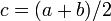
- Example
- Solve
 for
for  . Look for a root on the interval [0,1].
We proceed as follows:
- Write the equation in residual form:

- Determine the interval that we want to search for the root.
| Error creating thumbnail: Unable to save thumbnail to destination
|
{| | Iteration | a | b | c | residual |
|---|---|---|---|---|---|---|
| 1 | 0.0 | 1.0 | 0.5 | 0.36 | ||
| 2 | 0.5 | 1.0 | 0.75 | -0.27 | ||
| 3 | 0.5 | 0.75 | 0.625 | 0.0089 | ||
| 4 | 0.625 | 0.75 | 0.6875 | -0.15 | ||
| 5 | 0.625 | 0.6875 | 0.6562 | -0.072 | ||
| 6 | 0.6250 | 0.6562 | 0.6406 | -0.032 | ||
| 7 | 0.6250 | 0.6406 | 0.6328 | -0.012 | ||
| 8 | 0.6250 | 0.6328 | 0.6289 | -0.0016 |
| }
Regula Falsi
Open Domain Methods
|
Secant Method
Newton's Method
Solving a System of Nonlinear Equations
|
Newton's Method
Solution Approaches: Single Nonlinear Equation
Excel
To solve a nonlinear equation in Excel, we have to options:
- Goal Seek is a simple way to solve a single nonlinear equation.
- Solver is a more powerful way to solve a nonlinear equation. It can also perform minimization, maximization, and can solve systems of nonlinear equations as well.
Goal Seek
|
Solver
|
Matlab
To solve a single nonlinear equation in Matlab, we use the fzero function. If, however, we are solving for the roots of a polynomial, we can use the roots function. This will solve for all of the polynomial roots (both real and imaginary).
ROOTS
The roots function can be used to obtain all of the roots (both real and imaginary) of a polynomial
xroots = roots( coefs );
- coefs are the polynomial coefficients, in descending order.
- xroots is a vector containing all of the polynomial roots.
For example, consider the quadratic equation  . From the
quadratic formula,
we can identify the roots as
. From the
quadratic formula,
we can identify the roots as
where  is the imaginary number.
Using the roots function we have
x = roots( [3 -2 1] );
which gives
 x =
  0.3333 + 0.4714i
  0.3333 - 0.4714i
This is equivalent to the answer above obtained via the quadratic formula.
FZERO
In Matlab, fzero is the most flexible way to find the roots of a nonlinear equation. Its syntax is slightly different depending on the type of function we are using:
- For a function stored in an m-file named myFunction.m we use
x = fzero( 'myFunction', xguess );
- For an anonymous function named fun>/tt>
x = fzero( fun, xguess );
- For a built in function (like <tt>sin, exp, etc.)
x = fzero( @sin, xguess );
Note that fzero can only find real roots. Therefore, if we
tried to use it on the quadratic function , it
would fail. To demonstrate its usage, let's solve for the roots of the
function
From the quadratic formula, or by factoring this equation, we know
that its roots should be  and
and  .
.
To use fzero to solve this, we could use an anonymous function:
f = @(x)(3*x.^2-2*x-1);
x1 = fzero( f, -2 ); % start looking for the root at -2.0
x2 = fzero( f,  2 ); % start looking for the root at 2.0
This results in x1=-0.33333 and x2=1. Note that here we found the two roots by using different initial guesses. Of course it helps to know where the roots are so that you can supply decent initial guesses!
To solve this using a m-file, first create the function you will use:
function y = myQuadratic(x)
y = 3*x.^2 - 2*x -1
|
Save this in a file myQuadratic.m and then use fzero:
x1 = fzero( 'myQuadratic', -2.0 );  % start looking for the root at -2.0
x2 = fzero( 'myQuadratic',  2.0 );  % start looking for the root at 2.0
FMINSEARCH
Occasionally we want to maximize or minimize a function. Matlab provides a tool called fminsearch to do this. It searches for the minimum of a function near a starting guess. As with fzero, you use this in different ways depending on what kind of function you are minimizing:
 x = fminsearch( 'myFun', xo );  % when using a function in an m-file
 x = fminsearch( myFun,   xo );  % when using an anonymous function
 x = fminsearch( @myFun,  xo );  % when using a built-in function
|
Solution Approaches: System of Nonlinear Equations
|
Excel
Solver...
Matlab
fsolve