Regression
Contents
Introduction
Often time we measure some observable  as a function
of some independent variable,
as a function
of some independent variable,  , and we have some
theoretical function that we expect the observations to obey. The
function may have parameters in it that we need to determine. The
process of determining the best values of the parameters that fit the
function to the given data is known as regression.
, and we have some
theoretical function that we expect the observations to obey. The
function may have parameters in it that we need to determine. The
process of determining the best values of the parameters that fit the
function to the given data is known as regression.
Example
Consider the Arrhenius equation commonly used to describe the rate constant in chemistry,
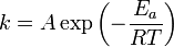
where
-
 is the rate constant of the chemical reaction,
 -
 is the pre-exponential factor
 -
 is the activation energy,
 -
 is the gas constant
 -
 is the temperature.
If we measured as a function of we could
determine and using regression.
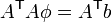
Linear Least Squares Regression
Linear Least Squares Regression can be applied if we can write our
function in polynomial form,  . If we can do this, then we are looking for
the coefficients of the polynomial,
. If we can do this, then we are looking for
the coefficients of the polynomial,  given
given
 observations
  . We can write
this as
. We can write
this as
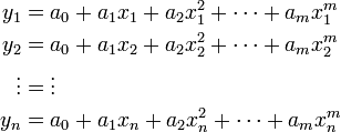
or, in matrix form,
![\underbrace{ \left[ \begin{array}{ccccc}
1 & x_1 & x_1^2 & \cdots & x_1^m \\
1 & x_2 & x_2^2 & \cdots & x_2^m \\
\vdots & \vdots & \cdots & \vdots \\
1 & x_n & x_n^2 & \cdots & x_n^m
\end{array} \right] }_{A}
\underbrace{ \left( \begin{array}{c}
a_0 \\ a_1 \\ a_2 \\ \vdots \\ a_m
\end{array}\right) }_{\phi}
=
\underbrace{ \left( \begin{array}{c}
y_1 \\ y_2 \\ \vdots \\ y_n
\end{array}\right) }_{b}](/wiki/images/math/1/7/f/17ffd709a9583bb9a1eff21ac104d0da.png)
Regression applies when  . In other words, when we have
many more equations than we have unknowns. In this case, the
least-squares solution is written as
. In other words, when we have
many more equations than we have unknowns. In this case, the
least-squares solution is written as
Example
Let's illustrate linear least squares regression with our example above. First, we must rewrite the problem:
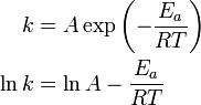
Note that this now looks like a polynomial, 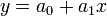 ,
where
,
where  ,
,  ,
,
 , and
, and  .
.
If we write these equations for each of our data points
in matrix form we obtain
![\underbrace{ \left[ \begin{array}{cc}
1 & \frac{-1}{RT_1} \\ 1 & \frac{-1}{RT_2} \\ 1 & \frac{-1}{RT_3} \\ \vdots & \vdots \\ 1 & \frac{-1}{RT_n}
\end{array} \right] }_{A}
\underbrace{ \left(\begin{array}{c}
a_0 \\ a_1
\end{array}\right) }_{\phi}
\underbrace{ \left(\begin{array}{c}
\ln k_1 \\ \ln k_2 \\ \ln k_3 \\ \vdots \\ \ln k_n
\end{array}\right) }_{b}](/wiki/images/math/d/3/4/d34d5ee3cdd529666d7bd2e54e8293c2.png)
and the equations to be solved are
Note that since is a 2x matrix and
 is a x1 vector, we have a 2x2 system of
equations to solve (see notes on
matrix multiplication).
is a x1 vector, we have a 2x2 system of
equations to solve (see notes on
matrix multiplication).
Example 2
Let's consider another example, where we want to determine the value
of the gravitational constant,  , via regression. To do
this, we could drop an object from a set height,
, via regression. To do
this, we could drop an object from a set height,  at
time
at
time  and measure its height as a function of time.
Neglecting air resistance, we have
and measure its height as a function of time.
Neglecting air resistance, we have
where  m/s2 is the gravitational
constant. Assume that
m/s2 is the gravitational
constant. Assume that  meters is known precisely,
and that since we drop the ball from rest,
meters is known precisely,
and that since we drop the ball from rest,  m/s. The
data we collect is given in the table below:
m/s. The
data we collect is given in the table below:
| time (s) | 0.08 | 0.28 | 0.48 | 0.53 | 0.70 | 1.05 | 1.31 | 1.36 |
| h(m) | 9.90 | 9.58 | 8.86 | 8.76 | 7.58 | 4.71 | 1.47 | 1.01 |
Let's go through this problem by hand:
- First, we rearrange our equation as follows:
 .
.
- Write down the equations in matrix form, one equation for each of
the data points.
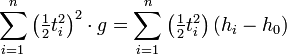
- Forming the normal equations, we have
 ,
,
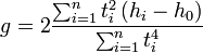
- Using the rules of
matrix multiplication, we
can rewrite this as
- Substituting numbers in from our above table, we obtain g=-9.75 m/s2
![\underbrace{
\left[\begin{array}{c}
\tfrac{1}{2}t_1^2 \\ \tfrac{1}{2}t_2^2 \\ \vdots \\ \tfrac{1}{2}t_n^2
\end{array} \right]
}_{A}
\underbrace{
\left( g \right)
}_{\phi}
=
\underbrace{
\left( \begin{array}{c}
h_1-h_0 \\ h_2-h_0 \\ \vdots \\ h_n-h_0
\end{array} \right)
}_{b}](/wiki/images/math/b/8/f/b8f1a423ad791da1da528f1be764c184.png)
![\left[\begin{array}{cccc}
\tfrac{1}{2}t_1^2 & \tfrac{1}{2}t_2^2 & \cdots & \tfrac{1}{2}t_n^2
\end{array} \right]
\left[\begin{array}{c}
\tfrac{1}{2}t_1^2 \\ \tfrac{1}{2}t_2^2 \\ \vdots \\ \tfrac{1}{2}t_n^2
\end{array} \right]
\left( g \right)
=
\left[\begin{array}{cccc}
\tfrac{1}{2}t_1^2 & \tfrac{1}{2}t_2^2 & \cdots & \tfrac{1}{2}t_n^2
\end{array} \right]
\left( \begin{array}{c}
h_1-h_0 \\ h_2-h_0 \\ \vdots \\ h_n-h_0
\end{array} \right)](/wiki/images/math/2/e/4/2e4fc204015375feffb9dd75968db57e.png)
Converting a Nonlinear Problem Into a Linear One
|
The R-Squared Value
The  value is a common way to measure how well a predicted value matches the observed data. It is calculated as
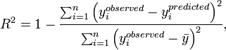
where  is a predicted value of
 ,
,  is the observed
value, and
is the observed
value, and 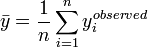 is the average value of the observed value of
.
is the average value of the observed value of
.
The value is always less than unity,  .
.
Nonlinear Least Squares Regression
The discussion and examples above focused on linear least squares regression, where the problem could be recast as a polynomial and we were solving for the coefficients of that polynomial. We showed an example of the Arrhenius equation which was originally nonlinear in the parameters but we rearranged it to be solved using linear regression.
Occasionally, it is not possible to reduce a problem to a linear one in order to perform regression. In such cases, we must use nonlinear regression, which involves solving a system of nonlinear equations for the unknown parameters.
Derivation of the Linear Least Squares Equations
|