Difference between revisions of "Linear Systems in Matlab"
m (→Solving Linear Systems of Equations in MATLAB) |
(→Example) |
||
| Line 12: | Line 12: | ||
=== Example === | === Example === | ||
| − | + | ||
| + | Consider the following set of equations: | ||
<center><math> | <center><math> | ||
\begin{cases} | \begin{cases} | ||
6y = -5x \\ | 6y = -5x \\ | ||
y = -3x -5 | y = -3x -5 | ||
| − | \end{cases} | + | \end{cases}. |
</math></center> | </math></center> | ||
| − | + | These can be easily solved by hand to obtain | |
| + | <math>(x,y) = \left( \tfrac{30}{13}, \tfrac{25}{13} \right) </math>. | ||
| + | |||
| + | To solve the system of equations using MATLAB, first rewrite these in a matrix-vector form as | ||
<center><math> | <center><math> | ||
\begin{align} | \begin{align} | ||
| Line 30: | Line 34: | ||
\left( \begin{array}{c} 0 \\ -5 \end{array} \right) . | \left( \begin{array}{c} 0 \\ -5 \end{array} \right) . | ||
</math></center> | </math></center> | ||
| − | + | Once in matrix-vector form, the solution is obtained in MATLAB by using the following commands: | |
<source lang="matlab"> | <source lang="matlab"> | ||
A = [ 5 6; 3 1 ]; % define the matrix | A = [ 5 6; 3 1 ]; % define the matrix | ||
| Line 36: | Line 40: | ||
solution = A\b; % solve the system of equations. | solution = A\b; % solve the system of equations. | ||
</source> | </source> | ||
| − | In this example, <tt>solution</tt> is a column vector whose elements are <tt>x</tt> and <tt>y</tt>. | + | In this example, <tt>solution</tt> is a column vector whose elements are <tt>x</tt> and <tt>y</tt>: |
| + | <center><math> | ||
| + | \mathrm{solution} = \left[ \begin{array}{c} -2.3077 \\1.9231 \end{array} \right], | ||
| + | </math></center> | ||
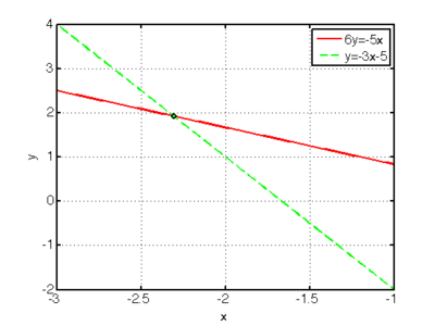
| + | which is consistent with the answer we obtained by hand above. The figure shows plots of the two equations, along with a circle indicating the solution (where the lines intersect). [[image:linsys_example.png|right|400px]] | ||
| + | |||
| + | |||
| + | ==== Matrix Inverse ==== | ||
Note that we can also form the inverse of a matrix, | Note that we can also form the inverse of a matrix, | ||
| Line 54: | Line 65: | ||
Ainv = inv(A); % entirely equivalent to A^-1. | Ainv = inv(A); % entirely equivalent to A^-1. | ||
</source> | </source> | ||
| − | |||
=== Sparse Systems === | === Sparse Systems === | ||
Revision as of 08:46, 25 August 2008
Contents
Solving Linear Systems of Equations in MATLAB
This section discusses how to solve a set of linear equations =(b)](/wiki/images/math/b/3/a/b3ae30ff4dcdb54b97d86d814ca503d6.png) in MATLAB.
See the discussion of linear algebra for help on writing a linear system of equations in matrix-vector format. There is also help on creating matrices and vectors in MATLAB.
in MATLAB.
See the discussion of linear algebra for help on writing a linear system of equations in matrix-vector format. There is also help on creating matrices and vectors in MATLAB.
The simplest way of solving a system of equations in MATLAB is by using the \ operator. Given a matrix A and a vector b, we may solve the system using the following MATLAB commands
x = A\b;
Example
Consider the following set of equations:

These can be easily solved by hand to obtain
 .
.
To solve the system of equations using MATLAB, first rewrite these in a matrix-vector form as
![\begin{align}
5x + 6y = 0 \\
3x + 1y &= -5 \\
\end{align}
\quad \Leftrightarrow \quad
\left[ \begin{array}{cc} 5 & 6 \\ 3 & 1 \end{array} \right]
\left( \begin{array}{c} x \\ y \end{array} \right) =
\left( \begin{array}{c} 0 \\ -5 \end{array} \right) .](/wiki/images/math/2/9/6/2965044b507f1faf6e68da9d984182e4.png)
Once in matrix-vector form, the solution is obtained in MATLAB by using the following commands:
  A = [ 5 6; 3 1 ];   % define the matrix
  b = [ 0; -5 ];      % define the vector
  solution = A\b;     % solve the system of equations.
In this example, solution is a column vector whose elements are x and y:
![\mathrm{solution} = \left[ \begin{array}{c} -2.3077 \\1.9231 \end{array} \right],](/wiki/images/math/e/5/0/e505e14fb2bca099016a128929a7e712.png)
Matrix Inverse
Note that we can also form the inverse of a matrix,
![[A] (x)=(b) \quad \Leftrightarrow \quad (x)=[A]^{-1}(b).](/wiki/images/math/9/6/0/96008bab47a724a093e8ed6374cec8f5.png)
This can be done in MATLAB as illustrated by the following:
  A = [ 5 6; 3 1 ];
  b = [ 0; -5 ];
  Ainv = A^-1;       % calculate the inverse of A
  solution = Ainv*b; % calculate the solution
We could also calculate A-1 by
Ainv = inv(A); % entirely equivalent to A^-1.
Sparse Systems
|
Linear Systems using the Symbolic Toolbox
Occasionally we may want to find the symbolic (general) solution to a system of equations rather than a specific numerical solution. The symbolic toolbox provides a way to do this.
|
