Nonlinear equations
Contents
Introduction
Nonlinear equations arise ubiquitously in science and engineering applications. There are several key distinctions between linear and nonlinear equations:
- Number of roots (solutions)
- For linear systems of equations there is a single unique solution for a well-posed system.
- For nonlinear equaitons there may be zero to many roots
- Solution Approach
- For linear systems, an exact solutions exist if system is well-posed
- For nonlinear systems, exact solutions are occasionally possible, but not in general. Solution methods are iterative.
Residual Form
Typically when solving a nonlinear equation we solve for its roots
- i.e. where the equation equals zero. In some cases we want to solve
an equation for where  . In such a case, we
must rewrite the equation in residual form:
. In such a case, we
must rewrite the equation in residual form:
Original Equation Residual Form 
For example, if we wanted to solve  for the
value of
for the
value of  where
where  , we would solve for the
roots of the function
, we would solve for the
roots of the function  .
.
Solving a Single Nonlinear Equation

There are two general classes of techniques for solving nonlinear equations:
- Closed domain methods - These methods look for a root inside a specified interval by iteratively shrinking the interval containing the root. These methods are typically more robust than open domain methods, but are somewhat slower to converge, and require that you be able to bracket the root.
- Open domain methods - These methods look for a root near a specified initial guess, but are not constrained in the region that they search for a root. These methods typically converge faster than closed domain methods, if the initial guess is "close enough" to the root.
Closed Domain Methods
Bisection
The bisection technique is fairly straightforward. Given an interval
![x=[a,b]](/wiki/images/math/c/6/a/c6a63bf83e1f74f471b7f59f12574f5b.png) that contains the root
that contains the root  , we
proceed as follows:
, we
proceed as follows:
- Set
 . We now have two intervals:
 ![[a,c]](/wiki/images/math/2/0/9/209f61583177d88b1f24c85f6a43c6ff.png) and
and ![[c,b]](/wiki/images/math/d/6/0/d6033df87877013a91e322ce6a5bc181.png) .
. - calculate

- choose the interval containing a sign change. In other words: if
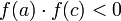 then we know a sign change occured on the interval and we select that interval. Otherwise we select the interval
 - Return to step 1.
The following Matlab code implements the bisection algorithm:
function x = bisect( fname, a, b, tol )
% function x = bisect( fname, a, b, tol )
% fname - the name of the function we are solving
% a - lower bound of interval containing the root
% b - upper bound of interval containing the root
% tol - solution tolerance (absolute)
  err = 10*tol;
  while err>tol
   fa = feval(fname,a);
   c = 0.5*(a+b);
   fc = feval(fname,c);
   err = abs(fc);
   if fc*fa<0
      % f(c) is of opposite sign from f(a).
      % This means that a and c now bracket
      % the root. Set up for the next pass.
      b = c;
   else
      % f(c) is of same sign as f(a). Thus, b and
      % c bracket the root. Set up for next pass.
      a = c;
   end end
  % set the return value x=0.5*(a+b);
- Example
- Solve
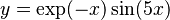 for
for  . Look for a root on the interval [0,0.4].
We proceed as follows:
- Write the equation in residual form:

- Set a=0, b=0.4. Calculate
 ,
,  .
. - Set
- evaluate
- Choose the sub-interval containing a sign change. This is the interval [a,c].
- Reset the interval: [a,b] = [0,0.2]
- return to step 3.
The plot for the first iteration is shown below, and the results for the first 9 iterations are also shown.
| Iteration | a | b | c | residual | |
|---|---|---|---|---|---|

|
1 | 0.0 | -0.4 | 0.2 | -0.19 |
| 2 | 0.0 | 0.2 | 0.1 | 0.066 | |
| 3 | 0.1 | 0.2 | 0.15 | -0.087 | |
| 4 | 0.1 | 0.15 | 0.125 | -0.016 | |
| 5 | 0.1 | 0.125 | 0.1125 | 0.023 | |
| 6 | 0.1125 | 0.125 | 0.1187 | 0.0032 | |
| 7 | 0.1187 | 0.1250 | 0.1219 | -0.0067 | |
| 8 | 0.1187 | 0.1219 | 0.1203 | -0.0018 | |
| 9 | 0.1187 | 0.1203 | 0.1195 | 0.00069 |
Regula Falsi
The Regula Falsi method is a simple variation on the
bisection method that is meant to improve convergence.
Rather than bisecting the interval into two equal halves (setting
c=(a+b)/2), we draw a line connecting  and
and
 and set c to the value of x
where the line crosses zero. Specifically,
and set c to the value of x
where the line crosses zero. Specifically,
- Calculate the slope of the line connecting and ,
- Calculate
- Choose the interval where the sign change occurs
- return to step 1.
The figure below illustrates this for the same function we considered
previously,  and the
first several iterations are shown.
and the
first several iterations are shown.
| Iteration | a | b | c | residual | |
|---|---|---|---|---|---|

|
1 | 0.0 | -0.4 | 0.3281 | -0.22 |
| 2 | 0.0 | 0.3281 | 0.2283 | -0.224 | |
| 3 | 0.0 | 0.2283 | 0.1578 | -0.11 | |
| 4 | 0.0 | 0.1578 | 0.1302 | -0.032 | |
| 5 | 0.0 | 0.1302 | 0.1124 | -0.0082 | |
| 6 | 0.0 | 0.1224 | 0.1204 | -0.0020 | |
| 7 | 0.0 | 0.1204 | 0.1199 | -0.00409 |
Comparing the results here with those from the bisection method, we see that the Regula Falsi method converges faster.
Open Domain Methods
Open domain methods do not require an interval that bounds the solution. Rather, they require an initial guess for the solution and refine that guess until convergence is achieved. Here we consider the secant method and Newton's method.
Secant Method
The secant method requires two initial guesses for the solution. In contrast to the closed domain methods, these guesses do not need to bracket the root. Given two guesses a and b, the algorithm is
- Calculate the slope of the line connecting and , .
- Calculate the point where this line is zero: .
- Check for convergence. If we are not converged, set a=b,
b=c and return to step 1.
On the function we considered previously,
 , with initial guesses of
0 and 0.4, the following table shows the
iteration:
, with initial guesses of
0 and 0.4, the following table shows the
iteration:
| Iteration | a | b | c | residual |
|---|---|---|---|---|
| 1 | 0.0000 | 0.4000 | 0.3281 | -0.22 |
| 2 | 0.4000 | 0.3281 | 0.4722 | 0.061 |
| 3 | 0.3281 | 0.4722 | 0.4407 | -0.019 |
| 4 | 0.4722 | 0.4407 | 0.4482 | -0.00068 |
The results here illustrate an important point. We converged to a different answer than we did using the bisection and regula falsi techniques! Try initial guesses of 0.0 and 0.1 and see what happens then...
Newton's Method
Newton's method is a bit more sophisticated than the secant method. It is also more robust and converges faster. It requires a single guess, but it also requies the function's derivative.
Newton's method is derived from a Taylor series expansion of a function. It gives the following result:
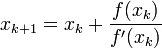
where  and
and  are the guesses for
the root at iteration k and k+1 respectively.
are the guesses for
the root at iteration k and k+1 respectively.
We have two options to evaluate  :
:
- Use an analytic expression. This is best but not always possible.
- Use numerical differentiation. In this case, we only need the function itself and we can approximate its derivative.
Returning to our example of solving
- ,
we have
 .
.
If we use an initial guess of x=0.2 then the values for x are:
|
|
Solving a System of Nonlinear Equations
When solving systems of nonlinear equations we are looking for the intersection of the equations. We can write a system of nonlinear equations as
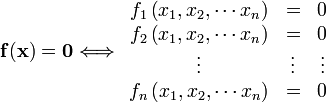
Newton's Method for Systems of Equations
For a system of nonlinear equations, Newton's method is written in matrix form as
or
![\left[\begin{array}{cccc}
J_{11} & J_{12} & \cdots & J_{1n}\\
J_{21} & J_{22} & \cdots & J_{2n}\\
\vdots & \vdots & \ddots & \vdots\\
J_{n1} & J_{n2} & \cdots & J_{nn}\end{array}\right]\left(\begin{array}{c}
\Delta x_{1}\\
\Delta x_{2}\\
\vdots\\
\Delta x_{n}\end{array}\right)=-\left(\begin{array}{c}
f_{1}(x_{1},x_{2},\cdots x_{n})\\
f_{2}(x_{1},x_{2},\cdots x_{n})\\
\vdots\\
f_{n}(x_{1},x_{2},\cdots x_{n})\end{array}\right)](/wiki/images/math/4/8/9/489db208e2407b3d598a3d0b0bc7e06d.png)
Here,  represents the change in all of
the variables at this iteration. The
represents the change in all of
the variables at this iteration. The ![[\mathbf{J}]](/wiki/images/math/0/a/d/0ad2c2c44fbd9ec9282f5b1769a30c70.png) matrix
is called the Jacobian matrix and is defined as
matrix
is called the Jacobian matrix and is defined as
In other words, it is the partial derivative of the ith function with respect to the jth independent variable.
Given a guess for the solution, the algorithm for Newton's method is
- Calculate the elements of the Jacobian matrix,
 .
. - Calculate the function values at the current value for
 ,
, 
- Solve the system of equations
![\left[\mathbf{J}\right]\left(\Delta\mathbf{x}\right)=-\mathbf{f}(\mathbf{x})](/wiki/images/math/7/0/5/705626b8d9d7325c8861e398a764f14f.png) for
for - Update the solution by adding to the current value of .
- Check for convergence. If not converged then go to step 1.
Example: Solve the system of equations
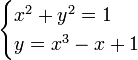
We can rewrite these as
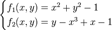
We need to be able to calculate the Jacobian. We do this as:
![J=
\left[\begin{array}{cc}
\frac{\partial f_{1}}{\partial x} & \frac{\partial f_{1}}{\partial y}\\
\frac{\partial f_{2}}{\partial x} & \frac{\partial f_{2}}{\partial y}
\end{array}\right]
=
\left[\begin{array}{cc}
2x & 2y\\
-3x^{2}+1 & 1
\end{array}\right]](/wiki/images/math/7/9/9/7994b82373c8de66b808e75cbcbe89f1.png)
Now we are ready to solve the system of equations.
|
| ||||||||||||||||||||||||||||||||||||||||||||||||||||||||||||||||||||||||||||
|

Note that there are two solutions to the system of equations, but in
the results above we only found one of the two roots. The root at
(x,y)=(0,1) was not found. You can verify that this is a
root by substituting it into the original equations and seeing that it
satifies both equations. Note that if we evaluate the Jacobian at
(0,1), we obtain ![J=\left[\begin{smallmatrix} 2 & 2\\ 1 &
1\end{smallmatrix}\right]](/wiki/images/math/3/c/3/3c3751e949148697a765c942b19ff71b.png) . This matrix cannot be inverted since the
second row is a multiple of the first. This illustrates problems that
Newton's method can run into.
. This matrix cannot be inverted since the
second row is a multiple of the first. This illustrates problems that
Newton's method can run into.
Solution Approaches: Single Nonlinear Equation
Excel
To solve a nonlinear equation in Excel, we have to options:
- Goal Seek is a simple way to solve a single nonlinear equation.
- Solver is a more powerful way to solve a nonlinear equation. It can also perform minimization, maximization, and can solve systems of nonlinear equations as well.
Goal Seek
|
Solver
|
Matlab
To solve a single nonlinear equation in Matlab, we use the fzero function. If, however, we are solving for the roots of a polynomial, we can use the roots function. This will solve for all of the polynomial roots (both real and imaginary).
ROOTS
The roots function can be used to obtain all of the roots (both real and imaginary) of a polynomial xroots = roots( coefs );
- coefs are the polynomial coefficients, in descending order.
- xroots is a vector containing all of the polynomial roots.
For example, consider the quadratic equation  . From the quadratic formula, we can identify the roots as
 where
where  is the imaginary number.
x = roots( [3 -2 1] );
 x =
  0.3333 + 0.4714i
  0.3333 - 0.4714i
This is equivalent to the answer above obtained via the quadratic formula.
FZERO
In Matlab, fzero is the most flexible way to find the roots of a nonlinear equation. Its syntax is slightly different depending on the type of function we are using:
- For a function stored in an m-file named myFunction.m we use
x = fzero( 'myFunction', xguess );
- For an anonymous function named fun>
x = fzero( fun, xguess );
- For a built in function (like sin, exp, etc.)
x = fzero( @sin, xguess );
Note that fzero can only find real roots. Therefore, if we tried to use it on the quadratic function , it would fail. To demonstrate its usage, let's solve for the roots of the function
From the quadratic formula, or by factoring this equation, we know that its roots should be  and
and  .
.
To use fzero to solve this, we could use an anonymous function:
f = @(x)(3*x.^2-2*x-1); x1 = fzero( f, -2 ); % start looking for the root at -2.0 x2 = fzero( f, 2 ); % start looking for the root at 2.0
This results in x1=-0.33333 and x2=1. Note that here we found the two roots by using different initial guesses. Of course it helps to know where the roots are so that you can supply decent initial guesses!
To solve this using a m-file, first create the function you will use: {| border="1" cellpadding="5" cellspacing="0" |+ style="background:lightgrey" | myQuadratic.m |-
| function y = myQuadratic(x) y = 3*x.^2 - 2*x -1
x1 = fzero( 'myQuadratic', -2.0 ); % start looking for the root at -2.0 x2 = fzero( 'myQuadratic', 2.0 ); % start looking for the root at 2.0
FMINSEARCH
Occasionally we want to maximize or minimize a function. Matlab provides a tool called fminsearch to do this. It searches for the minimum of a function near a starting guess. As with fzero, you use this in different ways depending on what kind of function you are minimizing:
 x = fminsearch( 'myFun', xo ); % when using a function in an m-file
 x = fminsearch( myFun, xo ); % when using an anonymous function
 x = fminsearch( @myFun, xo ); % when using a built-in function
|
Solution Approaches: System of Nonlinear Equations
|
Excel
Solver...
Matlab
fsolve