Numerical Differentiation
Introduction
Often we need to approximate the derivative of a function when we cannot obtain it analytically. Here we discuss several ways to do this numerically.
Taylor Series
Let's consider the situation where we have samples of a function
 at discrete points
  seperated by spacing
 as depicted in the following figure:

Consider a Taylor series expansions about some
arbitrary point  . Since
  we can write these as follows:
Approximation location Taylor Series Expansion about


If we subtract the Taylor series expansion at
from the one at , we find

Now we solve this for  to find
Now if is small, then the second term (with the
 in it) is small and we can approximate the derivative
as
in it) is small and we can approximate the derivative
as
We call this a second order approximation to
 because when we truncated the series
approximation to the largest term there was
of the order of .
because when we truncated the series
approximation to the largest term there was
of the order of .
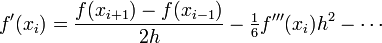
Note that we now have a way to approximate the derivative of a function if we have the function's values at two locations.
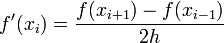
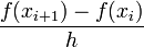
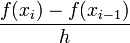
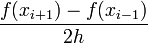
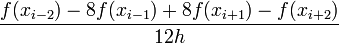
On a uniform mesh, we can use this technique to generate a variety of approximations to derivatives, as summarized in the following table:
|
 Error in approximation of  as a function of the size of the interval . Click here to download the matlab file that produced this plot. as a function of the size of the interval . Click here to download the matlab file that produced this plot. |


As can be seen in the figure above, higher order approximations result
in significantly lower error for a given spacing . Note
that for  the fourth-order approximation is
contaminated by roundoff error. The same would happen for the other
derivative approximations, but at smaller .
the fourth-order approximation is
contaminated by roundoff error. The same would happen for the other
derivative approximations, but at smaller .
Lagrange Polynomials
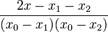
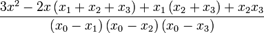
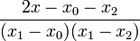
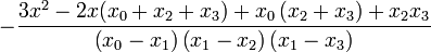
Lagrange polynomials, which are commonly used for interpolation, can also be used for differentiation. The formula is
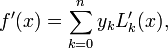
where  is given as
![L_{k}^{\prime}(x) = \left[ \sum_{{j=0}\atop{j\ne k}}^{n} \left( \prod_{ {i=0}\atop{i \ne j,k} }^n (x-x_i) \right) \right] \left[ \prod_{{i=0}\atop{i\ne k}}^{n} (x_k-x_i) \right]^{-1}.](/wiki/images/math/3/c/c/3cced1f629b2f0354163c2308a6df53c.png)
Here  is the order of the polynomial and we require
  points to form the Lagrange polynomial.
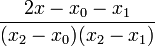
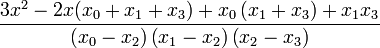
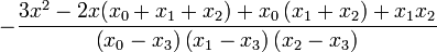
Here are the results for n = 2, 3, 4
n=2 n=3 n=4