Matlab Loops

Motivating Example

Suppose you wanted to create a program to see how often a given number turns up in Craps. If we roll two dice, the smallest number that can arise is 2, and the largest is 12. While there are more clever ways of doing this using probability, we take a brute-force method. Let's choose two random numbers between 1 and 6 and do this over again until we achieve the number we are betting on.

bet = 4; % the number we are looking for (between 2 and 12) dice = round( rand(2,1)*5+1 ); % two numbers between 1 and 6 if ( sum(dice) != bet ) % now what??? end

The problem is that we want to keep rolling the dice until we get our number (4 in this case). How do we do this? We use loops. There are two kinds of loops: for loops and while loops.

For Loops

A for loop is executed a set number of times. The basic syntax of a for loop is:

 for counter = lo:inc:hi
   % do some work
 end

counter	A variable that ranges from lo to hi
lo	Indicates the starting point for the counter
hi	Indicates the stopping point for the counter
inc	Indicates the increment for the counter. You can increment forward, backward, and in any size increment.

Each time through the loop, the counter variable will increment by inc. The loop exits when the counter exceeds hi. The following table shows several simple examples of a for loop.

Examples of using for loops

Matlab Code	Details	Output
for i=5:8 disp(i); end	i Action 5 Prints 5 6 Prints 6 7 Prints 7 8 Prints 8	5 6 7 8
x = 1:7; for i=2:2:length(x) x(i) = 2*x(i); end disp(x);	i Action 2 x(2) was 2, it is now 4 4 x(4) was 4, it is now 8 6 x(6) was 6, it is now 12	1 4 3 8 5 12 7
x = 3:7; for i=length(x):-2:1 fprintf('x(%1.0f) = %1.0f\n',i,x(i)); end	i Action 5 Prints: x(2) = 7 3 Prints: x(4) = 5 1 Prints: x(1) = 3	x(5) = 7 x(3) = 5 x(1) = 3

Factorial Example

Let's consider another example: calculate the factorial of a number using a for loop. The factorial is given as

$n! = \prod_{i=2}^{n} i\left(i-1\right)$

We could implement this using a for loop as shown in the following:

Matlab Code	Results at the end of each pass through the for loop
n = 7; % we want to find n! nfact=1; % starting value. for i=n:-1:2 nfact = nfact * i; end	Value of i 6 5 4 3 2 Value of nfact 6 30 120 360 720

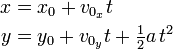
Projectile Motion Example

Suppose that we want to examine the effect of the angle on the path of a projectile. The equations for projectile motion (neglecting air resistance) can be written as

$\begin{align} x &= x_0 + v_{0_x} t \\ y &= y_0 + v_{0_y} t + \tfrac{1}{2}a\,t^2 \end{align}$

Assuming that the ground is level and that we launch from the point $(x,y)=(0,0)$, the projectile will hit the ground again when $y=0$. From the above equation for $y$, we conclude that this happens at $t=0$ and $t=-2 v_{0_y} / a$.

Let's create a Matlab script that will plot the trajectory of a projectile over the time of flight until it reaches the ground again. Here is an algorithm:

1. Set the initial speed, $v_0$
2. Set a vector of angles, $\theta$, that we want to consider.
3. For Each Angle:
   1. Calculate $v_{0_x}$ and $v_{0_y}$.
   2. Calculate the time of flight, $t=-\frac{2 v_{0_y}}{a}$
   3. Calculate the $x$ and $y$ positions over the time of flight and add these to the plot.
4. Label the plot.

This algorithm may be implemented in Matlab as follows:

clear; clc; close all; vo = 100; % initial velocity, m/s a = -9.8; % acceleration, m/s^2 angle = 5:10:85; % angles in degrees angle = angle*pi/180; % convert to radians figure; hold on; % create a figure and hold it for multiple lines. % loop over each angle and create the plot for its trajectory. for i=1:length(angle) vox = vo*cos( angle(i) ); % initial x-velocity for this angle voy = vo*sin( angle(i) ); % initial y-velocity for this angle tf = -2*voy/a; % time of flight for this angle t = linspace(0,tf); % a vector of time points for our plot. x = vox * t; % x-position at each point in time. y = voy * t + 0.5*a*t.^2; % y-position at each point in time. plot( x, y ); % plot this trajectory. % annotate the plot by adding a label to the line at the peak of the % trajectory indicating the angle that this line corresponds to. % find the index for the max height. There may be more than one if % we had a point on either side of the maximum. In this case, % choose the first one. maxpt = find( y==max(y) ); if( length(maxpt)>1 ) maxpt=maxpt(1); end; text( x(maxpt), y(maxpt), num2str(angle(i)*180/pi) ); end grid on; axis tight; xlabel('x (m)'); ylabel('y (m)'); title('Projectile Trajectories at Various Angles');

See notes on plotting and building arrays for explanations of those topics used in the above example.

This code produces the following plot:

Exponential Decay Example

Compounds undergoing [http://en.wikipedia.org/wiki/Exponential_decay exponential decay] obey the following equation, which describes the concentration, $c$ as a function of time:

$c = c_0 \exp\left( -k\, t \right),$

where $k$ is the time constant. This is often used in carbon dating. The half life is defined as the time required for the concentration to decrease by half. Using the previous equation, and substituting $c=c_0/2$ we find

$t_\mathrm{half} = -\ln(2)/k.$

Use Matlab to create a plot of the concentration as a function of time for various values of $k$. Indicate the half life on the plot. Assume that the initial concentration is $c_0=10.2$ (arbitrary units).

An algorithm may be:

1. Define a vector for $k$
2. Calculate the half life from the above equation for each $k$.
3. Determine how long in time to plot. Let's go twice the longest half life.
4. For Each value of $k$,
   1. Calculate $c$ as a function of $t$.
   2. Plot $c$ as a function of $t$.
   3. Put a point indicating the half life on the plot.
5. Label the plot

Below is the matlab code to implement the above algorithm. If you have questions about plotting, see the tutorial on plotting in matlab.

clear; clc; close all; k = [0.1 0.2 0.5 1]; % set the rate constants thalf = -log(0.5)./k; % determine half life for each rate constant t = linspace(0,max(thalf*2)); % set the time over which we will calculate c co = 10.2; % set the initial concentration figure; hold on; % loop over each rate constant. Plot its concentration % profile as well as the half-life time. for i=1:length(k); c = co*exp(-k(i)*t); plot(t,c); % plot the c vs time line plot(thalf(i),co/2,'rs'); % plot the point where we reach the half-life end plot(t,co/2*ones(length(t)),'r-'); % plot the half-life horizontal line % label the plot xlabel('time'); ylabel('Concentration'); title('Concentration vs. Time for Various Rate Contsants'); grid on; axis tight;

The results of this are shown in the following figure:

While Loops

Unlike a for loop (which is executed a set number of times), the while loop continues to execute until some condition is met. The basic syntax of a while loop is:

while condition % do some work. Note that "condition" must change inside the loop! end

Factorial Example

Here is an example of how to calculate the factorial of a number using a while loop.

Matlab Code	Results at the end of each pass through the while loop
n = 7; % we want to find n! nfact=1; % starting value. while n>1 nfact = nfact*n n = n-1 end	Iteration Number 1 2 3 4 5 6 Value of n 6 5 4 3 2 1 Value of nfact 7 42 210 840 2520 5040

Craps Example

Here is another example of rolling two dice. We keep rolling the dice until we get them to add up to 7. We print out how many rolls it took.

clear; clc; luckyNum = 7; % our lucky number. lucky = 0; % 0 is "false" - we will use this to determine when we hit our lucky number. nrolls = 0; % keep track of how many times we roll the dice. while ~lucky % pick 2 random integers between 1 and 6. The "round" function rounds to the nearest integer. dice = round( rand(2,1)*5+1 ); nrolls = nrolls+1; % increment the counter for how many rolls we have done. lucky = sum(dice)==luckyNum; % decide if we rolled a lucky 7 or not... end fprintf('Rolled a lucky %1.0f after %1.0f rolls\n',luckyNum,nrolls);

Here we have used the ~ operator, which is the logical "NOT" operator.