Interpolation
Contents
Linear Interpolation
A linear function may be written as 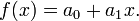 Given any two data points,
  , and
, and
 , we can determine a linear function that
exactly passes through these points. We can do this by solving for
, we can determine a linear function that
exactly passes through these points. We can do this by solving for
 and
and  . Since there are two unknowns we
require two equations. They are:
. Since there are two unknowns we
require two equations. They are:
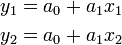
These may be written in matrix form as
![\left[ \begin{array}{cc}
1 & x_1 \\
1 & x_2
\end{array} \right]
\left( \begin{array}{c}
a_0 \\ a_1
\end{array} \right) =
\left( \begin{array}{c}
y_1 \\ y_2
\end{array} \right)](/wiki/images/math/8/9/d/89d586401931241c16145d9dbb27201a.png)
Given values for , and
, these equations may be easily
solved in MATLAB. But since they are so
simple, we can solve them by hand to obtain a general solution,
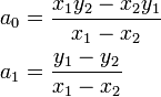
This gives the coefficients, which may then be substituted into the
original equation  and simplified to
obtain
and simplified to
obtain
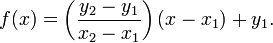
This is a very convenient equation for performing linear interpolation.
Example
The density of air at various temperatures and atmospheric pressure is given in the following table
| Temperature (°F) | -9.7 | 80 | 170 | 260 | 350 | 440 | 530 | 620 | 710 | 800 | 890 | 980 | 1070 |
|---|---|---|---|---|---|---|---|---|---|---|---|---|---|
| Density (kg/m3) | 1.39 | 1.16 | 0.99 | 0.87 | 0.78 | 0.69 | 0.63 | 0.58 | 0.54 | 0.50 | 0.46 | 0.44 | 0.41 |
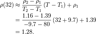
Estimate the density of air at 32 °F. Using linear interpolation,
we have  . We define
(T1, ρ1) = (-9.7, 1.39) and
(T2, ρ2) = (80, 1.161). Now we can calculate
. We define
(T1, ρ1) = (-9.7, 1.39) and
(T2, ρ2) = (80, 1.161). Now we can calculate
Implementation in Matlab
There are three ways to do linear interpolation in MATLAB.
- Form and solve the linear system. This is a simple 2x2 system since we only need to solve for the slope and intercept (two coefficients)
 T1=-9.7;  T2=80;
 rho1=1.39; rho2=1.16;
 T = 32;
 A = [ 1 T1; 1 T2 ];
 b = [ rho1; rho2 ];
 a = A\b;
 rho = a(1) + a(2)*T;
- Use the general equation we derived above. This is basically solving the linear system analytically and using the result to do the interpolation.
 T1=-9.7; T2-80;
 rho1=1.39; rho2=1.16;
 T = 32;
 rho = (rho2-rho1)/(T2-T1) * (T-T1) + rho1;
- Use MATLAB's built-in interpolation tool, interp1:
 Ti = [-9.7 80];
 rhoi = [1.39 1.16];
 rho = interp1( Ti, rhoi, 32 );
All three of these methods provide exactly the same answer. However, using MATLAB's interp1 function allows you to use a vector for the points that you want to interpolate to. For example, if we wanted the density at 30, 50, 70, 10, and 110 °F, we could accomplish this by:
  Ti = [-9.7 80 170 ];
  rhoi = [1.39 1.16 0.995];
  T = 30:20:110;
  rho = interp1( Ti, rhoi, T );
Polynomial Interpolation
Polynomial interpolation is a simple extension of linear interpolation. In general, an nth degree polynomial is given as
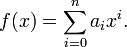
If n=1 then we recover a first-degree polynomial, which is
linear. The formula gives 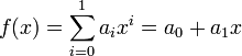 .
.
In general, if we want to interpolate a set of data using an
nth degree polynomial, then we must determine
n+1 coefficients,  . Therefore,
we require n+1 points to interpolate using an
nth degree polynomial.
. Therefore,
we require n+1 points to interpolate using an
nth degree polynomial.
The equations that must be solved are given as
![\left[\begin{array}{ccccc}
1 & x_{1} & x_{1}^2 & \cdots & x_{1}^{n}\\
1 & x_{2} & x_{2}^2 & \cdots & x_{2}^{n}\\
\vdots & \vdots & \vdots & \cdots & \vdots \\
1 & x_{n+1} & x_{n+1}^2 & \cdots & x_{n+1}^{n}
\end{array}\right]
\left(\begin{array}{c}
a_{0}\\ a_{1}\\ \vdots\\ a_{n}
\end{array}\right)
=
\left(\begin{array}{c}
y_{1}\\ y_{2}\\ \vdots\\ y_{n+1}
\end{array}\right)](/wiki/images/math/5/d/e/5dec415feed2a5970262778546fd8a82.png)
Solving these equations provides the values for the coefficients,
. Once we know these coefficients, we can
evaluate the polynomial at any point.
Example
Using a third degree (cubic) polynomial and the data in the table above, approximate the density of air at 50 °F and 300 °F.
A third degree polynomial (cubic polynomial) has four coefficients,
 . To determine these
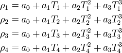
coefficients we require four equations. Assuming that we have four
observations for
. To determine these
coefficients we require four equations. Assuming that we have four
observations for  , the equations to be solved are:
Once we have solved these equations we have the polynomial coefficients and we can then evaluate the resulting polynomial at any temperature that we wish.
We still must choose what 4 points in the table to use in the above equations. We will choose the 4 points in the table that are closest to the temperature that we wish to interpolate to. Note that if we want to evaluate the density at different temperatures, we may want to use different points in the table to determine the coefficients!
Our procedure to perform the interpolation is:
- Determine which points we need to use.
- Set up and solve the linear system to obtain the polynomial coefficients
 .
. - Evaluate the polynomial to obtain the temperature.
Implementation in Matlab
The MATLAB code to obtain the density at 50 °F is
% Set the data points from the table.
Ti = [ -9.7   80  170  260  350  440  530 ...
        620  710  800  890  980 1070 ]';
rhoi=[ 1.39 1.16 0.99 0.87 0.78 0.69 0.63 ...
       0.58 0.54 0.50 0.46 0.44 0.41 ]';

% Set the temperature we want to evaluate the density at.
T = 50;

% determine the set of points that we will use to construct
% the interpolant. We want to use points that are closest
% to the temperature that we are interested in.
points = 1:4;

% set up the linear system
A = [ ones(4,1), ones(4,1).*Ti(points), ones(4,1)*Ti(points).^2, ones(4,1)*Ti(points).^3 ];
b = rhoi(points);

% solve for the polynomial coefficients
a = A\b;

% evaluate the density.
rho = a(0) + a(1)*T + a(2)*T^2 + a(3)*T^3;
For T=300 we would probably want to choose a different set of points to determine the polynomial coefficients. Therefore, we would repeat the above with the only change being:
 T=300;
 points=4:8;
Polynomial Interpolation in Matlab
Matlab has a command polyfit that can be used to fit a polynomial to data. Its syntax is
a = polyfit( x, y, order );
- x - the independent variable vector.
- y - the dependent variable vector.
- order - the order of the polynomial to fit the data to.
Note: for  data points, we can fit an
 order polynomial. However, Matlab will
allow you to use an order that is less than
order polynomial. However, Matlab will
allow you to use an order that is less than  . In the
case where you use an order less than , Matlab will
apply regression to determine the polynomial
coefficients. In this case, the resulting polynomial will not
necessarily interpolate the data points!
. In the
case where you use an order less than , Matlab will
apply regression to determine the polynomial
coefficients. In this case, the resulting polynomial will not
necessarily interpolate the data points!
Once you have the polynomial coefficients from polyfit, you can evaluate the polynomial easily using the polyval command:
yinterp = polyval( a, xinterp );
- a - the polynomial coefficients obtained from polyfit
- xinterp - the independent variable values we want to interpolate to.
- yinterp - the interpolated values.
Example
% Set the data points from the table.
Ti = [ -9.7   80  170  260  350  440  530 620  710  800  890  980 1070 ]';
rhoi=[ 1.39 1.16 0.99 0.87 0.78 0.69 0.63 0.58 0.54 0.50 0.46 0.44 0.41 ]';

% Set the temperature we want to evaluate the density at.
T = 50;

% fit the data to a polynomial.  We will use a third order polynomial.
% Therefore, we require four points.  We choose the points nearest T=50.
% If we used all of the data and a third order polynomial, we would end
% up with regression, not interpolation...
points = 1:4;
a = polyfit( x(points), y(points), 3 );

% interpolate to T=50:
rho = polyval( T, a );

% print out the result:
fprintf('The density at %.1f F is: %.2f kg/m^3\n',T,rho);
Cubic Spline Interpolation
Cubic spline interpolation uses cubic polynomials to interpolate datasets. The concept is illustrated in the following figure:

The data points are connected with cubic functions, and on each
interval the coefficients must be determined. If we have
data points then we can define cubic
functions, one between each data point. For each spline we have four
coefficients to determine. Therefore, we require  constraints to determine the coefficients.
The constraints may be summarized in the following table:
| Description | Mathematical Statement | Number of Constraints |
|---|---|---|
| At each data point, two splines meet. Here the splines must be equal to the data values. | 
|

|
| At the first and last point, the function must equal the data. | 
|

|
| At each interior point the first derivatives of adjacent splines must be equivalent. | 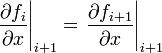
|

|
| At each interior point, the second derivatives of adjacent splines must be equivalent. | 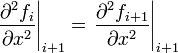
|
|
| We specify the curvature at the end points. By choosing the curvature to be equal to zero, we obtain a natural spline. | 
|
|

Adding up all of the constraints, we see that we have
constraints - precisely the number that we need.
We could formulate equations for all of these constraints and solve
them all to determine the coefficients for the cubic function on each
interval.
Example 1
Using the data in the table above, determine the density of air at the following temperatures: 60, 120, 180, 240, 300, 360, 420, 480, 540 °F.
Implementation in Matlab
Matlab has built-in functions for cubic spline interpolation:
y = interp1( xi, yi, x, 'spline' );
- (xi,yi) are the points at which we have data defined.
- x is the point(s) where we want to interpolate.
- 'spline' tells Matlab to interpolate using cubic splines.
Using this built-in function, we may obtain the interpolated values as follows:
% Set the data points from the table.
Ti = [ -9.7   80  170  260  350  440  530 ...
        620  710  800  890  980 1070 ]';
rhoi=[ 1.39 1.16 0.99 0.87 0.78 0.69 0.63 ...
       0.58 0.54 0.50 0.46 0.44 0.41 ]';

% set the temperatures that we want to interpolate to.
T = 60:60:540;

% determine the density at the desired temperatures.
rho = interp1( Ti, rhoi, T, 'spline' );
Lagrange Polynomial Interpolation
|
Given  points
  the
the
 order Lagrange polynomial that interpolates
these function values,
order Lagrange polynomial that interpolates
these function values,  are expressed as
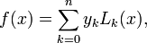
where  is the Lagrange polynomial given by
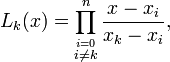
and  . In other words, for an
order interpolation, we require
points.
. In other words, for an
order interpolation, we require
points.
The  operator represents the continued product, and
is analogous to the
operator represents the continued product, and
is analogous to the  operator for summations. For
example,
operator for summations. For
example, 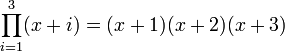 .
.