Difference between revisions of "Linear Systems in Matlab"
m |
m |
||
| (2 intermediate revisions by the same user not shown) | |||
| Line 5: | Line 5: | ||
This section discusses how to solve a set of linear equations <math>[A](x)=(b)</math> in MATLAB. | This section discusses how to solve a set of linear equations <math>[A](x)=(b)</math> in MATLAB. | ||
| − | See the discussion of [[ | + | See the discussion of [[Linear_Algebra|linear algebra]] for help on writing a linear system of equations in matrix-vector format. There is also help on [[Matlab_Arrays#Creating Arrays in Matlab|creating matrices and vectors]] in MATLAB. |
The simplest way of solving a system of equations in MATLAB is by using the '''\''' operator. Given a matrix '''A''' and a vector '''b''', we may solve the system using the following MATLAB commands: | The simplest way of solving a system of equations in MATLAB is by using the '''\''' operator. Given a matrix '''A''' and a vector '''b''', we may solve the system using the following MATLAB commands: | ||
<source lang="matlab"> | <source lang="matlab"> | ||
| − | x = A\b; | + | x = A\b; % Solve the linear system Ax=b for x. |
</source> | </source> | ||
| Line 24: | Line 24: | ||
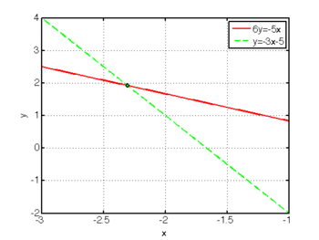
<math>(x,y) = \left( -\tfrac{30}{13}, \tfrac{25}{13} \right) </math>. These equations and their solution (intersection) are [[:Matlab_Plotting#X-Y_Line_Plots|plotted]] in the figure to the right. | <math>(x,y) = \left( -\tfrac{30}{13}, \tfrac{25}{13} \right) </math>. These equations and their solution (intersection) are [[:Matlab_Plotting#X-Y_Line_Plots|plotted]] in the figure to the right. | ||
| − | To solve the system of equations using MATLAB, first [[ | + | To solve the system of equations using MATLAB, first [[Linear_Algebra#Linear_Systems_of_Equations|rewrite these in a matrix-vector form]] as |
<center><math> | <center><math> | ||
\begin{align} | \begin{align} | ||
| Line 43: | Line 43: | ||
In this example, <tt>solution</tt> is a column vector whose elements are <tt>x</tt> and <tt>y</tt>: | In this example, <tt>solution</tt> is a column vector whose elements are <tt>x</tt> and <tt>y</tt>: | ||
<center><math> | <center><math> | ||
| − | \mathrm{solution} = \left[ \begin{ | + | \mathrm{solution} = \left[ \begin{smallmatrix}-2.3077 \\1.9231 \end{smallmatrix} \right], |
</math></center> | </math></center> | ||
which is consistent with the answer we obtained by hand above. | which is consistent with the answer we obtained by hand above. | ||
| Line 66: | Line 66: | ||
Ainv = inv(A); % entirely equivalent to A^-1. | Ainv = inv(A); % entirely equivalent to A^-1. | ||
</source> | </source> | ||
| − | |||
=== Sparse Systems === | === Sparse Systems === | ||
{{Stub|section}} | {{Stub|section}} | ||
| − | |||
| − | |||
== Linear Systems using the Symbolic Toolbox == | == Linear Systems using the Symbolic Toolbox == | ||
Latest revision as of 08:14, 26 August 2009
Contents
Solving Linear Systems of Equations in MATLAB
This section discusses how to solve a set of linear equations =(b)](/wiki/images/math/b/3/a/b3ae30ff4dcdb54b97d86d814ca503d6.png) in MATLAB.
See the discussion of linear algebra for help on writing a linear system of equations in matrix-vector format. There is also help on creating matrices and vectors in MATLAB.
in MATLAB.
See the discussion of linear algebra for help on writing a linear system of equations in matrix-vector format. There is also help on creating matrices and vectors in MATLAB.
The simplest way of solving a system of equations in MATLAB is by using the \ operator. Given a matrix A and a vector b, we may solve the system using the following MATLAB commands:
x = A\b; % Solve the linear system Ax=b for x.
Example
Consider the following set of equations:
These can be easily solved by hand to obtain
 . These equations and their solution (intersection) are plotted in the figure to the right.
To solve the system of equations using MATLAB, first rewrite these in a matrix-vector form as
![\begin{align}
5x + 6y &= 0 \\
3x + 1y &= -5 \\
\end{align}
\quad \Leftrightarrow \quad
\left[ \begin{array}{cc} 5 & 6 \\ 3 & 1 \end{array} \right]
\left( \begin{array}{c} x \\ y \end{array} \right) =
\left( \begin{array}{c} 0 \\ -5 \end{array} \right) .](/wiki/images/math/1/7/4/174e63aeefd5db446681be987bdadb7e.png)
Once in matrix-vector form, the solution is obtained in MATLAB by using the following commands (see here for help on creating matrices and vectors):
  A = [ 5 6; 3 1 ];   % define the matrix
  b = [ 0; -5 ];      % define the vector
  solution = A\b;     % solve the system of equations.
In this example, solution is a column vector whose elements are x and y:
![\mathrm{solution} = \left[ \begin{smallmatrix}-2.3077 \\1.9231 \end{smallmatrix} \right],](/wiki/images/math/d/3/c/d3c5261fb7a5b071957c0d2e6109bc9b.png)
which is consistent with the answer we obtained by hand above.
Matrix Inverse
Note that we can also form the inverse of a matrix,
![[A] (x)=(b) \quad \Leftrightarrow \quad (x)=[A]^{-1}(b).](/wiki/images/math/9/6/0/96008bab47a724a093e8ed6374cec8f5.png)
This can be done in MATLAB as illustrated by the following:
  A = [ 5 6; 3 1 ];
  b = [ 0; -5 ];
  Ainv = A^-1;       % calculate the inverse of A
  solution = Ainv*b; % calculate the solution
We could also calculate A-1 by
Ainv = inv(A); % entirely equivalent to A^-1.
Sparse Systems
|
Linear Systems using the Symbolic Toolbox
Occasionally we may want to find the symbolic (general) solution to a system of equations rather than a specific numerical solution. The symbolic toolbox provides a way to do this.
|
