Interpolation

Linear Interpolation

A linear function may be written as $f(x) = a_0 + a_1 x.$ Given any two data points, $( x_1, y_1 )$, and $(x_2,y_2)$, we can determine a linear function that exactly passes through these points. We can do this by solving for $a_0$ and $a_1$. Since there are two unknowns we require two equations. They are:

$\begin{align} y_1 &= a_0 + a_1 x_1 \\ y_2 &= a_0 + a_1 x_2 \end{align}$

These may be written in matrix form as

$\left[ \begin{array}{cc} 1 & x_1 \\ 1 & x_2 \end{array} \right] \left( \begin{array}{c} a_0 \\ a_1 \end{array} \right) = \left( \begin{array}{c} y_1 \\ y_2 \end{array} \right)$

Given values for $( x_1, y_1 )$, and $(x_2,y_2)$, these equations may be easily solved in MATLAB. But since they are so simple, we can easily by hand to obtain a general solution,

$\begin{align} a_0 &= \frac{x_1 y_2 -x_2 y_1}{x_1-x_2} \\ a_1 &= \frac{y_1-y_2}{x_1-x_2} \end{align}$

This gives the coefficients, which may then be substituted into the original equation $f(x) = a_0 + a_1 x$ and simplified to obtain

$f(x) = \left( \frac{y_2-y_1}{x_2-x_1} \right) \left( x-x_1 \right) + y_1.$

This is a very convenient equation for performing linear interpolation.

Example

The density of air at various temperatures and atmospheric pressure is given in the following table

Temperature (°F)	1.39	1.16	0.99	0.87	0.78	0.69	0.63	0.58	0.54	0.50	0.46	0.44	0.41
Density (kg/m3)	-10	80	170	260	350	440	530	620	710	800	890	980	1070

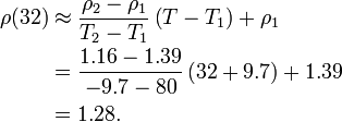
Estimate the density of air at 32 °F. Using linear interpolation, we have $\rho(T)=a_0 + a_1 T$. We define $(T_1,\rho_1)=(-9.7,1.39)$ and $(T_2,\rho_2)=(80,1.161)$. Now we can calculate

$\begin{align} \rho(32) &\approx \frac{\rho_2 -\rho_1}{T_2-T_1}\left( T - T_1 \right) + \rho_1 \\ &= \frac{1.16-1.39}{-9.7-80} \left( 32 + 9.7 \right) + 1.39 \\ &= 1.28. \end{align}$

Implementation in Matlab

There are three ways to do interpolation in MATLAB.

1. Solve the linear system.

    T1=-9.7;  T2=80;
    rho1=1.39; rho2=1.16;
    T = 32;
    A = [ 1 T1; 1 T2 ];
    b = [ rho1; rho2 ];
    a = A\b;
    rho = a(1) + a(2)*T;
   

2. Use the general equation we derived above:

    T1=-9.7; T2-80;
    rho1=1.39; rho2=1.16;
    T = 32;
    rho = (rho2-rho1)/(T2-T1) * (T-T1) + rho1;
   

3. Use MATLAB's built-in interpolation tool

    Ti = [-9.7 80];
    rhoi = [1.39 1.16];
    rho = interp1( Ti, rhoi, 32 );
   

All three of these methods provide exactly the same answer. However, using MATLAB's interp1 function allows you to use a vector for the points that you want to interpolate to. For example, if we wanted the density at 30, 50, 70, 10, and 110 °F, we could accomplish this by:

  Ti = [-9.7 80 170 ];
  rhoi = [1.39 1.16 0.995];
  T = 30:20:110;
  rho = interp1( Ti, rhoi, T );

Implementation in Excel

{{Stub}|section}}

Polynomial Interpolation

Polynomial interpolation is a simple extension of linear interpolation. In general, an n^th degree polynomial is given as $f(x)=\sum_{i=0}^n a_i x^i.$

If n=1 then we recover a first-degree polynomial, which is linear. The formula gives $f(x)=\sum_{i=0}^1 a_i x^i = a_0 + a_1 x$.

In general, if we want to interpolate a set of data using an n^th degree polynomial, then we must determine n+1 coefficients, $a_0 \ldots a_n$. Therefore, we require n+1 points to interpolate using an n^th degree polynomial.

The equations that must be solved are given as

$\left[\begin{array}{ccccc} 1 & x_{1} & x_{1}^2 & \cdots & x_{1}^{n}\\ 1 & x_{2} & x_{2}^2 & \cdots & x_{2}^{n}\\ \vdots & \vdots & \vdots & \cdots & \vdots \\ 1 & x_{n+1} & x_{n+1}^2 & \cdots & x_{n+1}^{n}\end{array}\right]\left(\begin{array}{c} a_{0}\\ a_{1}\\ \vdots\\ a_{n}\end{array}\right) = \left(\begin{array}{c} y_{1}\\ y_{2}\\ \vdots\\ y_{n+1}\end{array}\right)$

Solving these equations provides the values for the coefficients, $a_0 \ldots a_n$. Once we know these coefficients, we can evaluate the polynomial at any point.

Example

Using a third degree polynomial, approximate the density of air at the following temperatures: 50, 300, 500 °F.

We require 4 points to fit a third degree polynomial, $a_0 \, a_1 \, a_2 \, a_3$. We will choose the 4 points closest to the temperature that we wish to interpolate to.

Implementation in Matlab

Our procedure is:

1. Determine which points we need to use.
2. Set up and solve the linear system to obtain the polynomial coefficients $a_0 \ldots a_3$.
3. Evaluate the polynomial to obtain the temperature.

Ti = [ -9.7   80  170  260  350  440  530  620  710  800  890  980 1070 ]';
rhoi=[ 1.39 1.16 0.99 0.87 0.78 0.69 0.63 0.58 0.54 0.50 0.46 0.44 0.41 ]';

T = 50;
points = 1:4;
A = [ ones(4,1), ones(4,1).*Ti(points), ones(4,1)*Ti(points).^2, ones(4,1)*Ti(points).^3 ];
b = rhoi(points);
a = A\b;

rho = a(0) + a(1)*T + a(2)*T^2 + a(3)*T^3;

For T=300 we would repeat the above with the only change being:

T=300;
points=4:8;

For T=500 we would change

T=500;
points=5:9;

Cubic Spline Interpolation

This section is a stub and needs to be expanded. If you can provide information or finish this section you're welcome to do so and then remove this message afterwards.

Lagrange Polynomial Interpolation

Given $n_p$ points $(x_k,y_k),$ the $n^\mathrm{th}$ order Lagrange polynomial that interpolates these function values, $f(x)$ are expressed as

$f(x)=\sum_{k=0}^{n} y_{k} L_{k}(x),$

where $L_{k}(x)$ is the Lagrange polynomial given by

$L_{k}(x)=\prod_{\stackrel{i=0}{i\ne k}}^{n}\frac{x-x_{i}}{x_{k}-x_{i}},$

and $n_p = n+1$. In other words, for an $n^\mathrm{th}$ order interpolation, we require $n_p=n+1$ points.

The $\prod$ operator represents the continued product, and is analogous to the $\sum$ operator for summations. For example, $\prod_{i=1}^{3} (x+i) = (x+1)(x+2)(x+3)$.