Isothermal CSTR Reactor Simulation
By Taylor Geisler
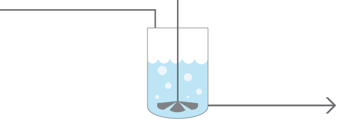
The Problem
In this example we will investigate an isothermal stirred tank reactor with a single, nonreversible reaction.
\(A+B\rightarrow C+D\)
The concentration over time of each species can be described by an ordinary differential equation. The ODE consists of terms accounting for flow in, flow out, generation, and consumption.
\(\frac{dN_{i}}{dt}=flow\: in-flow\: out+generation-consumption\)
Substituting the rate of reaction for the the generation and consumption terms we get
\(\frac{dN_{i}}{dt}=F_{i\, in}-F_{i\, out}+r_{i}V\)
Dividing by the volume of the reactor V we get the differential equation in terms of concentration.
\(\frac{dC_{i}}{dt}=\frac{\nu_{in}}{V}C_{i\, in}-\frac{\nu_{out}}{V}C_{i\, out}+r_{i}\)
Using this ODE we can solve for the reactor contents over time. The equations for each compenent are written here.
\(\frac{dC_{A}}{dt}=\frac{\nu_{in}}{V}C_{A\, in}-\frac{\nu_{out}}{V}C_{A\, out}+r_{A}\)
\(\frac{dC_{B}}{dt}=\frac{\nu_{in}}{V}C_{B\, in}-\frac{\nu_{out}}{V}C_{B\, out}+r_{B}\)
\(\frac{dC_{C}}{dt}=\frac{\nu_{in}}{V}C_{C\, in}-\frac{\nu_{out}}{V}C_{C\, out}+r_{C}\)
\(\frac{dC_{D}}{dt}=\frac{\nu_{in}}{V}C_{D\, in}-\frac{\nu_{out}}{V}C_{D\, out}+r_{D}\)
We will use the common irreversible rate equation
\(r_{A}=kC_{A}C_{B}\)
Where
\(r_{A}=r_{B}=-r_{C}=-r_{D}\)
We must know the initial concentrations in the reactor in order to solve the differential equations. Once we know these concentrations, we have everything we need to solve for the concentration over time.
The Solver
The Backward Euler method was used to solve the ordinary differential equations. This is an implicit time integrator that uses the derivative at time step j+1 to determine the change in concentration from time j to j+1.
\(C_{i\, j+1}=C_{i\, j}+\Delta t\frac{dC_{i\, j+1}}{dt}\)
Here is this equation written in residual form for each species. Notice that the differential expressions from above have been substituted for the differential.
\(f_{1}=-C_{A\, j+1}+C_{A\, j}+\Delta t\left(\frac{\nu_{in}}{V}C_{A\, in}-\frac{\nu_{out}}{V}C_{A\, j+1}+r_{A\, j+1}\right)\)
\(f_{2}=-C_{B\, j+1}+C_{B\, j}+\Delta t\left(\frac{\nu_{in}}{V}C_{B\, in}-\frac{\nu_{out}}{V}C_{B\, j+1}+r_{B\, j+1}\right)\)
\(f_{3}=-C_{C\, j+1}+C_{C\, j}+\Delta t\left(\frac{\nu_{in}}{V}C_{C\, in}-\frac{\nu_{out}}{V}C_{C\, j+1}+r_{C\, j+1}\right)\)
\(f_{4}=-C_{D\, j+1}+C_{D\, j}+\Delta t\left(\frac{\nu_{in}}{V}C_{D\, in}-\frac{\nu_{out}}{V}C_{D\, j+1}+r_{D\, j+1}\right)\)
We cannot solve these equations algebraically. Note that the r term is a nonlinear function of the product of \( C_{A} \) and \( C_{B} \).
To solve this nonlinear system of equations, Newton’s Method was employed at each time step. Newton’s method requires iteratively solving the equation
\(J\cdot\Delta x=-RHS\)
The terms J and RHS are constructed using the nonlinear equations that we are trying to solve.
\(
J=\begin{bmatrix}\frac{df_{1}}{dC_{A}} & \frac{df_{1}}{dC_{B}} & \frac{df_{1}}{dC_{C}} & \frac{df_{1}}{dC_{D}}\\
\frac{df_{2}}{dC_{A}} & \frac{df_{2}}{dC_{B}} & \frac{df_{2}}{dC_{C}} & \frac{df_{2}}{dC_{D}}\\
\frac{df_{3}}{dC_{A}} & \frac{df_{3}}{dC_{B}} & \frac{df_{3}}{dC_{C}} & \frac{df_{3}}{dC_{D}}\\
\frac{df_{4}}{dC_{A}} & \frac{df_{4}}{dC_{B}} & \frac{df_{4}}{dC_{C}} & \frac{df_{4}}{dC_{D}}
\end{bmatrix}
\)
\(
RHS=\begin{bmatrix}f_{1}(C_{A},C_{B},C_{C},C_{D})\\
f_{2}(C_{A},C_{B},C_{C},C_{D})\\
f_{3}(C_{A},C_{B},C_{C},C_{D})\\
f_{4}(C_{A},C_{B},C_{C},C_{D})
\end{bmatrix}
\)
\(
\Delta x=\begin{bmatrix}\Delta C_{A}\\
\Delta C_{B}\\
\Delta C_{C}\\
\Delta C_{D}
\end{bmatrix}
\)
First, a guess of \( C_{A\, j+1}\), \( C_{B\, j+1}\), \( C_{C\, j+1}\), and \( C_{D\, j+1} \) are required. The jacobian matrix J and the RHS vector are calculated. The derivatives in the jacobian matrix were calculated using the forward difference approximation.
Now that we have all the necessary terms, we can solve for the vector \( \Delta x\). This is a vector of updates to our initial guesses. We add these updates to our original guesses and reconstruct the jacobian and RHS terms with the new, better values. This process is repeated until the updates become small. This means that we have converged to the solution, within a given tolerance.
By repeating this process at each time step, we solve for \( C_{A}\), \( C_{B}\), \( C_{C}\), and \( C_{D} \) over time. The solution is plotted above.
The Simulation
Experiment with different values in the above simulation to see how the reaction will change. The simulation shows both inital reactor dynamics as well as the steady state values that are eventually reached. Experiment with changing the rate constant of the reaction to produce a higher or lower concentration of products at steady state. Adjust the flow rate and examine the change in the inital dynamics of the system. Examine how the steady state values react when you change the inlet concentration of one of the products or reactants.